Transient Simulation of a Metal Cooling Process.
Akpan, Patrick 1 and Njiofor, Tobenna 2
1 Department of Mechanical Engineering, University of Nigeria, Nsukka
2 Process Systems Engineering, Cranfield University, UK.
* E-mail of the corresponding author: Patrick.akpan@unn.edu.ng; +2348102475639
Abstract
Transient heat conduction is encountered in metallurgical industries where metals are subjected to different heat treatment processes to enhance their physical and chemical properties (e.g. annealing). The actual heat treatment process involves complex heat transfer processes described andsuch problems are preferentially solved using numerical methods. This work studies the transient cooling of a metal plate using a finite volume-based commercial CFD code. The temperature distribution in the metal plate during the cooling process was well predicted for both the explicit and implicit schemes with the maximum error occurring at the boundary nodes.At the constant heat flux boundary x=0, the numerical model under predicted the temperatures with a maximum error of −0.08%. At the convective boundary x=0.135 m, the numerical model over predicted the temperatures with a maximum error of 0.79%. Furthermore more computational time was required in the explicit scheme in contrast to the implicit scheme that required less time. Using the implicit scheme, the calculated time for the plate to attain steady state was approximately 47,000 s. Keywords: Transient simulation, metal cooling, CFD, finite volume and heat treatment.
INTRODUCTION
Transient or time dependent temperature fields appear when the thermal conditions at the boundaries of a body change (Holman, 2010). For instance, if a body with initial constant temperature is placed in an environment at a different temperature, then heat will flow over the surface of the body and its temperature will change over time. The governing equation for heat conduction in cartesian form obtained by applying the first law of thermodynamics to a differential control volume taken from a quiescent, isotropic and incompressible material with temperature dependent material property k(T) is is given in Eq. 1.The heat sources within the thermally conductive body are accounted for by the volumetric heat generation rate (W˙).
ρcp∂t∂T=div[k(T)gradT]+W˙(T,x,t)
Ultimately a new steady state condition will be reach at the end of this time dependent process. The solution of a transient heat conduction problem can be found in three different ways (Baehr and Stephan, 2006):
- By a closed solution of the heat conduction equation fulfilling all the boundary conditions.
- By an experimental method implementing an analogy process.
- By a numerical solution of the heat conduction equation with boundary conditions.
In order to find a closed solution by mathematical functions, the material properties must be assumed to be temperature independent (Cengel, 2003). To ensure that a linear differential equation is produced, the problem is often limited to either conduction without internal heat sources, or the heat generation rate is presupposed to be independent of or only linearly dependent on temperature. In addition, the boundary condition requires a constant or time dependent, but non-temperature dependent heat transfer coefficient h. The following methods have been used in obtaining closed form solutions: separation of variables, superimposing of heat sources and sinks, Green’s theorem and Laplace transformation.
Experimental analogy procedures are based on the fact that different transient processes, in particular electrical conduction, lead to partial differential equations which have the same form as the heat conduction equation. Study is made of an analogous process and the results are then transferred to the thermal conduction process. As a result of the extensive progress in computer technology, this method has very little practical importance today (Baehr and Stephan, 2006).
The numerical solution of a transient heat conduction problem is of particular importance when temperature dependent material properties or bodies with irregular shapes or complex boundary conditions, for example a temperature dependent h, are present. In such cases a numerical solution is generally the only choice of solution.
The application possibilities for numerical solutions haveincreased considerably since the introduction of computers. Computational Fluid Dynamics (CFD) numerical tools are based on any of these three discretization methods - finite difference (FD), finite element (FE), and finite volume (FV) (Blazek, 2001; Chung, 2002 and Njiofor, 2009) .
The FV method is a Control volume based technique of numerical discretisation. It offers several advantages (including its conservativeness and robustness) that make it particularly attractive for use in both academic and commercial CFD applications. It is also well suited for investigating diffusion problems. It implements the following computational steps: (a)Mesh generation entailing the division of the domain of interest into discrete control volumes, (b) Integration of the governing equations on the individual control volumes to construct algebraic equations for the discrete variables (the unknowns) such as pressure, velocity, temperature, and conserved scalars. © Linearization of the discretised equations and solution of the resulting linear system of equations to yield updated values of the dependent variables (Njiofor, 2009, Eymard et. al., 2000 and Versteeg and Malalasekara, 2007).
Heat treatment processes are used in metallurgical industries to enhance the physical and chemical properties (e.g. annealing) of metals. The heat treatment process involves complex heat transfer processes described by highly-nonlinear partial differential equation such that closed form solution can only be obtained by making simplifying assumptions. Such problems are preferentially solved using numerical methods.
This work studies the transient cooling of a metal plate using a finite volume-based commercial CFD code. The objective of this work is to demonstrate how to solve a transient conduction heat transfer problem by using a finite volume approach.
MATERIAL AND METHODS
The numerical simulation was done using a commercial CFD tool Ansys Fluent version 12.1 (Fluent Inc., 2006) and the results of the simulation were compared with analytical solutions.
Problem Description
The simplest problems in transient heat conduction are problems involving the calculation of a temperature field T=T(x,t), which changes with time only in the x− direction. A further requirement is that there are no sources of heat generation. Such problems are known as linear heat flow problems. A typical example is the annealing process. Annealing in metallurgy and material science is a heat treatment process that alters the properties of a material achieved by heating to above the re-crystallization temperature and maintaining at a suitable temperature, before cooling uniformly in a fluid. Here the interest is in the cooling process and the case to be investigated is the transient cooling of a steel plate.
The steel plate investigated is shown in Figure 1 and has thermal conductivity and diffusivity of 15 W/mK and 3.75×10⁻⁶ m2/s respectively. It is 270 mm thick and has a constant initial temperature, To=300∘C. At time t>0 the plate is brought into contact with a fluid which has a temperature Tf=20∘C that is constant with respect to time. The heat transfer coefficient at both surfaces of the plate is h=75 W/m2 K. The temperatures during the cooling of the plate are to be numerically determined. Simple initial and boundary conditions were intentionally chosen for comparison of results. Due to the symmetrical nature of the problem, it is sufficient to consider only one half of theplate i.e. xs=0.135 m (see Figure 1). Its left hand surface can be taken to be adiabatic, while heat is transferred to the surrounding fluid from the right surface.
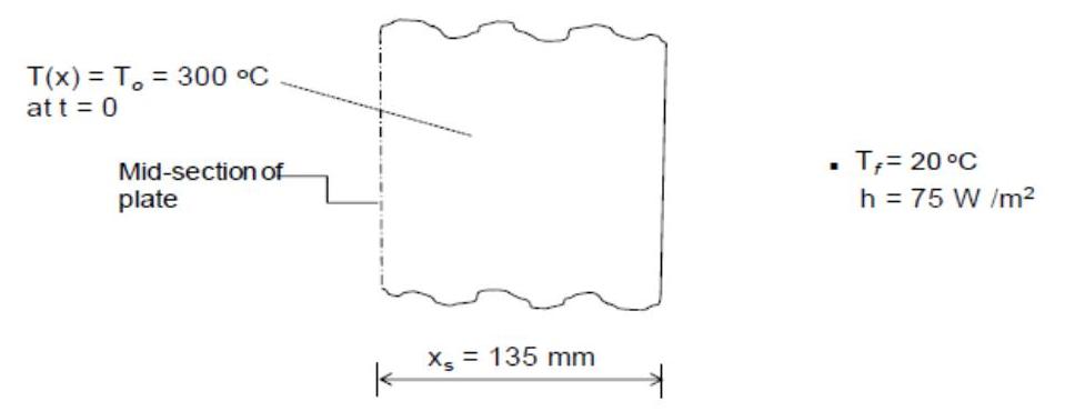
Figure 1 Schematic diagram of longitudinal section through the mid-section of the steel plate (Baehr and
Stephan, 2006)
Grid Generation and Simulation Details
The grid used for this work was generated using GAMBIT and measures 0.3 m×0.135 m (see Figure 2). The spacing between the nodes Δx is 0.015 m .
Boundary Conditions and Discretization
In Figure 2 the mid-section of the plate (surface AB ) was assigned a zero heat flux boundary condition (adiabatic plane). As the problem is one-dimensional, the two surfaces, BC and AD were also assigned zero heat flux while surface CD was assigned convective boundary condition with the heat transfer coefficientand fluid temperature set equal to 75 W/m2 K and 293.15 K(20∘C) respectively.

Figure 2 Steel plate geometrical grid model.
The central differencing scheme was used to discretize the diffusive fluxes in the heat conduction equation. The temperature at the nodes was initialized to 773.15 K(200∘C). Since the problem is unsteady, time marching was implemented using both the explicit and implicit schemes.
Explicit scheme
The time step for the first-order explicit method is subject to the condition (Badr, 2010 and Cengel, 2003) given in (Eq. 2) as:
Δt<ρcp2k(Δx)2<2π(Δx)2
Using this criterion, the limit on time step for time marching was determined as 30 s . A time step of 20 s was first used to run the simulation before using the value given by the limit so as to be able to compare the results obtained using a time step of 20 s to that obtained using 30 s time step. For each time step, convergence was declared when the normalized residual of the applicable heat diffusion equation (also energy equation) became less than 10−6.
Implicit scheme
As the implicit scheme is unconditionally stable, any time step can be used for it (Badr, 2010 and Cengel, 2003) . However, a time step of 20 s was first used to run the simulation before using 30 s in order to compare the results obtained using the two time steps and also compare results obtained with a time step of 30 s to that from the explicit scheme. Finally, convergence was declared when the normalized residual of the applicable heat conduction equation became less than 10−6 as was the case in the explicit scheme.
RESULTS AND DISCUSSION
The exact solution for the problem is given in Baehr and Stephan (2006)as
T(x,t)=Tf+[Te−Tf][i=1∑∞CiCas(λixgx)exp(−λi2xg2πt)]
Where xg is half the plate’s thickness, λi are the eigenvalues of the problem given by the roots of the equation.
Tωnλ=λπt
and Ci are coefficients calculated as
Ci=λi+sinλicosλi2sinλi
Explicit Scheme
The results for the first 15 consecutive time steps are shown in Table 1 while the contours of temperature plot at t =960 s is shown in Figure 3. It can be seen from Table 1 that the temperature of the steel plate decreased with each forward march in time. The temperature drop increased from the mid-section to the outer surface of the plate with the largest drops occurring at the boundary node in contact with the fluid. Also, a look at the table shows that the temperature response at nodes inside the plate is very minimal. This behavior is attributed to the relationship between the rate of change of temperature of the plate and its thermal diffusivity seen from the general heat conduction equation (Eq.1).
According to the equation, the change of temperature with time, ∂T/∂ε at each point inside the steel plate is proportional to the thermal diffusivity. Thus the thermal diffusivity has a direct effect on how quickly the temperature changes inside the plate and as its value is small in this case study ( 3.75×10⁻⁶ m2/s ), the rate of change of temperature will also be small. The contours of temperature plot (Figure 3) revealed the existence of temperature gradients in the plate, with the mid-section having the highest temperature.
A comparison of the numerical and analytical results at 320 s,640 s and 960 s from the start of the cooling process is illustrated graphically in Figure 4. The error analysis clearly shows that the results are in good agreement with the analytical solution except at the convective boundary where maximum error occurred. This can be attributed to the coarseness of the grid used for the computation. The use of fine grid around the nodes will further reduce the errors to very low values as fine grid captures the large temperature gradients occurring at boundary nodes better than coarse grid.
Table 1 Results showing temperature distribution in the plate (explicit method with time step of 20 s )
Time
step |
Time
(s) |
Distance from the mid-section to the outer surface of the plate |
|
|
|
|
|
|
|
|
|
|
|
|
|
|
|
x=0.0 |
x=0.015 |
x=0.045 |
x=0.075 |
x=0.105 |
x=0.135 |
| 0 |
0 |
573.15 |
573.15 |
573.15 |
573.15 |
573.15 |
573.15 |
| 1 |
20 |
573.15 |
573.15 |
573.15 |
573.12 |
572.49 |
562.95 |
| 2 |
40 |
573.15 |
573.15 |
573.14 |
573.04 |
571.45 |
558.77 |
| 3 |
80 |
573.15 |
573.15 |
573.13 |
572.89 |
570.19 |
555.25 |
| 4 |
100 |
573.15 |
573.15 |
573.11 |
572.66 |
568.81 |
552.21 |
| 5 |
120 |
573.15 |
573.14 |
573.06 |
572.36 |
567.38 |
549.52 |
| 6 |
140 |
573.14 |
573.13 |
573.01 |
571.99 |
565.94 |
547.09 |
| 7 |
160 |
573.13 |
573.12 |
572.92 |
571.56 |
564.50 |
544.88 |
| 8 |
180 |
573.12 |
573.10 |
572.82 |
571.08 |
563.08 |
542.83 |
| 9 |
200 |
573.10 |
573.08 |
572.69 |
570.55 |
561.69 |
540.93 |
| 10 |
220 |
573.08 |
573.04 |
572.54 |
569.99 |
560.33 |
539.15 |
| 11 |
240 |
573.04 |
573.00 |
572.36 |
569.39 |
559.00 |
537.48 |
| 12 |
260 |
573.00 |
572.94 |
572.16 |
568.77 |
557.71 |
535.89 |
| 13 |
280 |
572.95 |
572.87 |
571.94 |
568.13 |
556.45 |
534.38 |
| 14 |
300 |
572.89 |
572.79 |
571.70 |
567.47 |
555.22 |
532.95 |
| 15 |
320 |
572.81 |
572.69 |
571.43 |
566.80 |
554.03 |
531.57 |
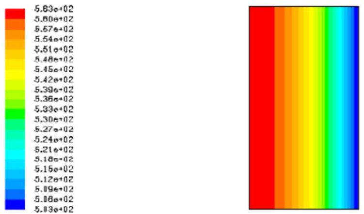
Figure 3 Contours of temperature at t=960 s (explicit method. time step 20 s )

Figure 4 Comparison of numerical and analytic solutions at different times (explicit method)

Figure 5 Comparison of result obtained using different time step values (explicit method)
Figure 5 compares the solution when time steps of 20 s and 30 s are used at time t=960 s. The previous result with a time step of 20 s and the exact solution are also shown for comparison. As the figure illustrates, there is
no significant difference between the values obtained for the 20 s and 30 s time steps as a result of the low temperature response of the plate.
Implicit Scheme
From Figure 6, it can be seen that the solution using implicit scheme compare favourably with analytical solution. In order to assess the performance of both the explicit and implicit schemes, the analytical solution together with explicit and implicit solutions at t=960 s obtained using a time step of 30 s is shown in Figure 7. Though the differences between the two methods in this case study were not significant due to the low thermal response of the plate, the explicit scheme is known to give unrealistic oscillations at any time step greater than the limit imposed by Eq. 2 while the implicit method tolerates much larger time steps.
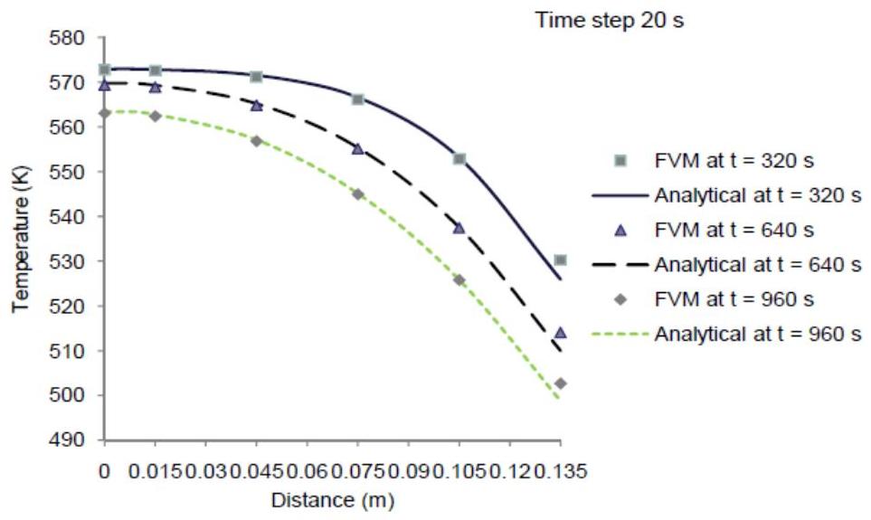
Figure 6 Comparison of numerical and analytical solutions at different times (implicit method)
For instance, simulation using the implicit scheme with a time step of 80 s gave results that compared favorably with analytical results as Table 2 illustrates though with higher error values as when compared to results obtained using a lower time step. This is the key advantage of the implicit scheme of time discretization.

Figure 7 Comparison of explicit and implicit solutions for time step of 30 s
Table 2 Comparison of numerical and analytical solutions at different times (implicit method at a time step 80s)
Distance
(m) |
Temperature |
|
|
|
|
|
|
|
|
|
Time =320 s |
|
|
Time =640 s |
|
|
Time =960 s |
|
|
|
FVM∗( K) |
Alt ∗∗( K) |
Error (%) |
FVM ∗( K) |
Alt ∗∗( K) |
Error (%) |
FVM ∗( K) |
Alt ∗∗( K) |
Error (%) |
| 0.000 |
572.40 |
572.94 |
−0.09 |
568.83 |
569.79 |
−0.17 |
562.66 |
563.47 |
−0.15 |
| 0.015 |
572.25 |
572.81 |
−0.10 |
568.39 |
569.29 |
−0.16 |
562.01 |
562.76 |
−0.13 |
| 0.045 |
570.76 |
571.50 |
−0.13 |
564.54 |
565.19 |
−0.12 |
556.67 |
557.11 |
−0.08 |
| 0.075 |
565.97 |
566.56 |
−0.10 |
555.28 |
555.34 |
−0.01 |
545.16 |
545.09 |
0.01 |
| 0.105 |
553.50 |
553.09 |
0.74 |
538.08 |
537.52 |
0.10 |
526.31 |
525.80 |
0.10 |
| 0.135 |
531.42 |
525.92 |
1.05 |
514.85 |
509.99 |
0.95 |
503.27 |
498.75 |
0.90 |
*FVM - Finite Volume Method results **Alt - Analytical results
However, since the accuracy of the implicit scheme used for this study is only first-order in time, realistic time steps are needed to ensure the accuracy of results. For the explicit scheme, it is very computational expensive to try to divide the computational grid into fine grid as the time step limit will also become very small. For example, with the division of the computational domain into 36 parts, the time step limit for the explicit scheme becomes 1.875 s which will require more computational time assuming that the temperature distribution at steady state is to be determined. This is the reason why the implicit scheme is recommended for general purpose transient calculations because of less computational time and unconditional stability. However, the implicit scheme requires more computer core memory as nodal equations are solved simultaneously at each time step in contrast to the explicit scheme where the nodal equations are solved sequentially at each time step.
Using the implicit scheme with a time step of 20 s , the transient temperature response of the steel plate for t>0 was calculated and the results for the two boundary nodes are shown in Figure 8. It can be seen from Figure 8 that the steel plate experienced steep negative temperature gradients from the commencement of the cooling process till about 20000 seconds later when marginal temperature gradients were observed. Further probing revealed that it took more than 13 hours for the plate to attain steady state. This means that the plate lost heat at a minimal rate due to the low convective heat transfer coefficient between it and the surrounding fluid.

Figure 8 Transient temperature response of the steel plate
CONCLUSION AND RECOMMENDATION
Conclusion
The finite volume method is well suited for studying transient heat conduction as it gives results that are very close to analytical ones (where they exist). The differences between results obtained using the explicit and implicit method of time discretization for the problem considered in this work were not much given the low temperature response of the plate. However, the explicit method has a time step limitation which makes it computational expensive for studying transient heat conduction problems in particular and CFD application in general where fine mesh is often used to run simulations.
The finite volume method having been successfully used to investigate simple diffusion problems can also be used to study heat conduction problems with no known exact solution (steady and unsteady multi-dimensional problems with complicated geometries and boundary conditions). However, it should be pointed out that the finite volume method being a numerical tool often requires a great deal of programming, memory, and computing time which should not be underestimated.
Recommendation
The heat conduction problem considered in this work was a simple heat transfer case. It was chosen for the purpose of comparison with analytical solutions. A thorough investigation of the suitability of the finite volume method for heat transfer problems involving heat transfer by conduction is being suggested for future work as there is currently limited treatment using the method in the literature. This willhelp to expand current knowledge on the method and also lead to further improvement of the method. Studies involving assessment of the performance of the three numerical discretization methods (finite difference, finite element and finite volume) in relation to the solution of heat transfer problems are also being proposed.
The central differencing scheme used in the discretization of the diffusive fluxes in the general transport equation is second-order accurate. In order to improve the accuracy of discretization process, differencing schemes with higher-order accuracy is needed hence it is being suggested that more research should be made towards developing differencing schemes with higher-order accuracy.
REFERENCES
Badr, O. (2010) Heat transfer lecture note: Presented at Cranfield University, UK. Unpublished.
Baehr, H. D. and Stephan, K. (2006). Heat and mass transfer, 2nd Ed. Springer, Berlin.
Blazek, J. (2001). Computational fluid dynamics: principles and applications. Elsevier Science, Oxford.
Cengel Y.A., Heat Transfer: A Practical Approach, 2nd ed., McGraw-Hill, 2003
Chung, T. J. (2002). Computational fluid dynamics.Cambridge University Press, Cambridge.
Eymard, R., Gallouet, T. and Herbin, R. (2000).Finite volume methods.Handbook of Numerical Analysis, 7, 713−1020.
Fluent Inc. (2006).Fluent 6.3 user guide documentation. Fluent Inc., Lebanon.
Holman, J. P. (2010). Heat Transfer, 10th Ed. McGraw-Hill, New York
Njiofor, M. T. (2009). Tool for numerical discretisation: finite Volume method for diffusion problems. Cranfield University, UK. MSc Thesis Unpublished.
Versteeg, H. K. and Malalasekera, W. (2007).An introduction to computational fluid dynamics: The finite volume method, 2nd Ed. Pearson Education, Harlow,England.
ACKNOWLEDGEMENT
The authors wish to thank the Nigerian government who through the Petroleum Technology Development Fund (PTDF) sponsored this research.
NOMENCLATURES
| Symbols |
Definition |
Units |
| ρ |
Density |
[Kg/m3] |
| cp |
Specific heat at constant pressure |
[J/kgK] |
| T |
Temperature |
[K] |
| t |
Time |
[s] |
| u |
Velocity |
[m/s] |
| x |
displacement in x rectangular coordinate |
[m] |
| k |
Thermal conductivity |
[W/mK] |
| W˙ |
Volumetric heat generation rate |
[W/m3] |
| h |
Heat transfer co-efficient |
[W/m2 K] |
| Tf |
Temperature of ambient fluid |
[K] |
| Tb |
Initial temperature of metal plate |
[K] |
| xs |
Half the metal plate thickness |
[m] |
| λi |
Eigenvalues of the problem |
[−] |
| Bι |
Biot number |
[−] |
 Patrick Akpan


