Meta-Cayley Graphs on Dihedral Groups

Meta-Cayley Graphs on Dihedral Groups

by
Imran Allie

A thesis submitted in fulfillment of the requirements for the degree of Master of Science, in the
Department of Mathematics and Applied Mathematics
University of Western Cape
UNIVERSITY of the
WESTERN CAPE

Supervised by
Prof Eric Mwambene

January 2017

Abstract

The pursuit of graphs which are vertex-transitive and non-Cayley on groups has been ongoing for some time. There has long been evidence to suggest that such graphs are a very rarety in occurrence. Much success has been had in this regard with various approaches being used. The aim of this thesis is to find such a class of graphs. We will take an algebraic approach. We will define Cayley graphs on loops, these loops necessarily not being groups. Specifically, we will define meta-Cayley graphs, which are vertex-transitive by construction. The loops in question are defined as the semidirect product of groups, one of the groups being $\mathbb{Z}_{2}$ consistently, the other being in the class of dihedral groups. In order to prove non-Cayleyness on groups, we will need to fully determine the automorphism groups of these graphs. Determining the automorphism groups is at the crux of the matter. Once these groups are determined, we may then apply Sabidussi’s theorem. The theorem states that a graph is Cayley on groups if and only if its automorphism group contains a subgroup which acts regularly on its vertex set.

Declaration

I hereby declare that this thesis is my own work, that it has not been submitted for any degree or examination at any other academic institution, and that all the sources I have used or quoted have been indicated and acknowledged by complete references.

Imran Allie
January 2017

Signed:

Acknowledgements

I would like to thank: my parents, for their support and encouragement; my wife, for her love and respect; my supervisor, for his time and mentorship.

I would also like to thank the Chemicals Industries Education and Training Authority (CHIETA) and the Student Enrolment Management Unit (SEMU) for awarding and administering to myself a bursary for this Masters degree.

Most importantly, all thanks is due to Allah, who has granted me the blessings mentioned above, and also the ability to be thankful to them and to him.

Contents

1 Introduction … 6
2 Preliminaries … 8
2.1 Basic graph theory … 8
2.2 Basic algebraic definitions … 11
3 Graphs on groupoids … 14
3.1 Cayley graphs … 14
3.2 Quasi-associativity … 17
3.3 Meta-Cayley graphs … 20
4 Constructing graphs on dihedral groups … 24
4.1 Constructing loops … 24
4.2 Meta-Cayley subsets … 28
5 Automorphism groups and non-Cayleyness … 39
5.1 Sabidussi’s theorem … 39

5.2 The graphs $\Omega(n, r)$ … 41
5.3 The graphs $\Gamma(n, r)$ … 43

UNIVERSITY of the WESTERN CAPE

Chapter 1

Introduction

Vertex-transitivity in graphs represents a measure of symmetry, which is defined by the graph having an automorphism group which acts transitively on the vertex set. Archetypal vertex-transitive graphs are those defined as Cayley graphs on groups.

While it can be proved, without difficulty, that all Cayley graphs on groups are vertex-transitive, the reverse implication does not hold. A counter example for the reverse implication is the well-known Petersen graph.

Through computational observations, it has been conjectured by Ivanov and Praeger [7] that

$$\lim _{n \rightarrow \infty} \frac{\operatorname{cay}(\mathrm{n})}{\operatorname{vtr}(\mathrm{n})}=1$$

where $\operatorname{vtr}(n)$ and $\operatorname{cay}(n)$ denote the number of isomorphism types of vertex-transitive and Cayley graphs on groups, respectively, with order at most $n \geq 1$. In other words, it is conjectured that the majority of vertex-transitive graphs are Cayley on groups. That is, the majority of vertex-transitive graphs can be represented by a group and a Cayley set. Much earlier, in [9] Marušič asked for which positive integers $n$ does there exist a vertex-transitive graph on $n$ vertices which is not Cayley on groups. It has been noted that there are indications that vertex-transitive graphs that are not Cayley on groups are a rarity in occurrence. Further, finding classes of graphs which are vertex-transitive and non-Cayley on groups has proved to be no simple matter. The determination of vertex-transitive graphs that are not Cayley on groups has thus raised a lot of attention. Notable success has been had in the construction

of such graphs; see, for instance, $[2,6,8,10,11,18,20]$. Much of the success had in this line has been in part due to Sabidussi’s theorem in [19]. The theorem states that a graph is Cayley on a group if and only if the automorphism group contains a subgroup which acts regularly on the vertex set.

The method of defining a Cayley graph on a group has been generalised to defining a Cayley graph on a groupoid in [13]. In fact, it was shown that every graph is representable on some groupoid. As mentioned, every Cayley graph on a group is vertex-transitive. However, to ensure vertex-transitivity of a Cayley graph on a groupoid, all we require is that the groupoid is a loop, and the Cayley set conforms to a property called quasi-associativity, a concept introduced by Gauyacq in [5].

In [16], meta-Cayley graphs were introduced. These graphs are vertex-transitive by construction. The construction involves the semi-direct product of two groups of which the twisting map satisfies a certain weak condition, such that the semi-direct product is a loop. Also, the Cayley set on the semi-direct product takes a particular form to ensure quasi-associativity. Of course this semi-direct product need not be a group. Thus, an avenue for the determination of vertex-transitive graphs which are non-Cayley on groups was introduced.

The purpose of this thesis is to define a class of meta-Cayley vertex-transitive graphs and then prove these graphs to be non-Cayley on groups. In Chapter 2, we present the necessary preliminaries relating to graph theory and groupoids. In Chapter 3 we explain how graphs are constructed on groupoids. Also, we present meta-Cayley graphs. In Chapter 4, we construct our vertex-transitive meta-Cayley graphs. In Chapter 5, we fully determine the automorphism groups of our constructed graphs and prove that they are non-Cayley on groups by applying Sabidussi’s theorem. Henceforth, we will refer to vertex-transitive graphs which are non-Cayley on groups by the acronym VTNCGs introduced by Watkins in [20].

Chapter 2

Preliminaries

In this chapter, we present the necessary preliminaries relating to graph and group theory. Naturally we begin with the formal definition of a graph. Thereafter, we define various concepts. At the crux of what we aim to achieve in this thesis is the determination of automorphism groups of graphs. Therefore, we define automorphisms on graphs which is also necessary in introducing the concept of vertex-transitivity. Also included are the definitions of certain algebraic structures, particularly groupoids and loops, as well as the semi-direct product of groups. We conclude the chapter with the definition of a class of graphs which we will consider in this thesis, that is, the generalised Petersen graphs.

2.1 Basic graph theory

Formally, graphs are defined as follows.
Definition 2.1. Let $V$ be a non-empty set and $E$ a relation on $V$. We call the pair $\Gamma=(V, E)$ a digraph. If $E$ is irreflexive and symmetric, we call the pair $\Gamma=(V, E)$ a graph.

In a graph $\Gamma=(V, E)$ the elements of $V$ are called vertices and the elements of $E$ are called edges. Edges are denoted as $[x, y]$ where $x, y \in V$. We say that $x$ and $y$ are adjacent, $x$ and $y$ are incident, or that $x$ and $y$ are neighbours. Similarly, edges

can also be thought of as incident or adjacent if they share a common vertex. The degree or valency of a vertex is the number of edges incident with it. If the degree is the same for each vertex in the graph, then we refer to the degree of the graph.

We now define various types of sequences of vertices.
Definition 2.2. Let $\Gamma=(V, E)$ be a graph.
(a) A walk is a sequence of vertices $v_{0}, v_{1}, \ldots, v_{k}$ such that $\left[v_{i}, v_{i+1}\right] \in E$ for every $i \in\{0,1, \ldots, k-1\}$. $k$ is called the length of the walk.
(b) A trail is a walk in which every edge is distinct.
© A path is a trail in which every vertex in $\left\{v_{0}, v_{1}, \ldots, v_{k-1}\right\}$ is distinct.
(d) A cycle is a path in which $v_{k}=v_{0}$. An $n$-cycle is a cycle with $n$ vertices.

Let $\Gamma=(V, E)$ be a graph. Define a relation $\sim$ on $V$ by $x \sim y$ if and only if there exists a path from $x$ to $y$. If $x \sim y$ then $x$ and $y$ are said to be connected. It is not hard to see that $\sim$ is an equivalence relation. Each equivalence class $[x]$ is called a component of the graph. If a graph has more than one component then it is disconnected, otherwise it is connected.

Graph homomorphisms can naturally be defined as mappings which preserve the relation on the vertex set. That is, graph homomorphisms are edge-preserving.

Definition 2.3. Let $\Gamma$ and $\Lambda$ be graphs. Let $\phi$ be a mapping, $\phi: V(\Gamma) \longrightarrow V(\Lambda)$.
(a) If $[x, y] \in \Gamma$ implies $[\phi(x), \phi(y)] \in \Lambda$ then $\phi$ is called a homomorphism. $\Gamma$ and $\Lambda$ are said to homomorphic.
(b) If $\phi$ is a bijective homomorphism and $\phi^{-1}$ is a homomorphism then $\phi$ is called an isomorphism. $\Gamma$ and $\Lambda$ are said to be isomorphic, denoted as $\Gamma \cong \Lambda$.
© If $\phi$ is an isomorphism from a graph to itself then $\phi$ is called an automorphism.

Remark 2.4. The automorphisms of a graph $\Gamma$ form a group under composition. The automorphism group is denoted as Aut $\Gamma$.

In this thesis, we will be proving isomorphic relations between graphs. We present the following lemma which will prove useful in this regard.

Lemma 2.5. Let $\Gamma$ and $\Lambda$ be graphs with finite vertex sets and let $\phi: V(\Gamma) \longrightarrow V(\Lambda)$ be a bijective homomorphism. If $|E(\Gamma)|=|E(\Lambda)|$ then $\Gamma \cong \Lambda$.

Proof. Let $E(\Gamma)=\left\{e_{1}, e_{2}, \ldots, e_{k}\right\}$. Then $\phi(E(\Gamma))=\left\{\phi\left(e_{1}\right), \phi\left(e_{2}\right), \ldots, \phi\left(e_{k}\right)\right\}$. For each $i$ let $e_{i}=\left[x_{i}, y_{i}\right]$ so that $\phi\left(e_{i}\right)=\left[\phi\left(x_{i}\right), \phi\left(y_{i}\right)\right]$. Since $\phi$ is a bijection on the vertex sets, each $\phi\left(e_{i}\right)$ is distinct. Therefore, $|E(\Lambda)|=|E(\Gamma)|=|\phi(E(\Gamma))|$ so that $\phi$ is onto with respect to edges. By the pigeonhole principle, $\phi^{-1}$ is a homomorphism so that $\phi$ is an isomorphism.

Remark 2.6. For automorphisms, the order of the edge sets are obviously the same. Thus we will not explicitly apply Lemma 2.5 when proving that certain maps are automorphisms.

Since the automorphisms form a group, we consider the action of this group on the set of vertices or edges. For any vertex $x \in V$ and automorphism $\gamma \in$ Aut $\Gamma$ we define the action of $\gamma$ on $x$ as $\gamma(x)$. Similarly for an edge $[x, y] \in E$ we define the action of $\gamma$ on $[x, y]$ as $\gamma([x, y])=[\gamma(x), \gamma(y)]$. If for any two vertices $x, y \in V$ there exists an automorphism $\gamma \in$ Aut $\Gamma$ such that $\gamma(x)=y$, then the group Aut $\Gamma$ is said to act transitively on $V$. If for any two edges $\left[x_{1}, y_{1}\right],\left[x_{2}, y_{2}\right] \in E$ there exists an automorphism $\gamma \in$ Aut $\Gamma$ such that $\gamma\left(\left[x_{1}, y_{1}\right]\right)=\left[x_{2}, y_{2}\right]$, then the group Aut $\Gamma$ is said to act transitively on $E$. This leads us to the definition of vertex-transitivity and edge-transitivity.

Definition 2.7. Let $\Gamma=(V, E)$ be a graph.
(a) If Aut $\Gamma$ acts transitively on $V(\Gamma)$ then $\Gamma$ is said to be vertex-transitive.
(b) If Aut $\Gamma$ acts transitively on $E(\Gamma)$ then $\Gamma$ is said to be edge-transitive.
© Let $H$ be a subgroup of Aut $\Gamma$ which acts transitively on $V(\Gamma)$. If $H$ has the same order as $V(\Gamma)$ then $H$ is said to act regularly on $V(\Gamma)$.

We immediately note that if a graph is vertex-transitive then every vertex has the same degree. Also, every vertex is contained in the same amount of cycles of each size. For these reasons, we think of vertex-transitivity as a measure of symmetry within graphs.

Let $\Gamma=(V, E)$ be a graph. Define a relation $\sim$ on $V$ by $x \sim y$ if and only if there exists an automorphism $\gamma \in$ Aut $\Gamma$ such that $\gamma(x)=y$. It is easy to see that $\sim$ is an

equivalence relation. The equivalence class containing a vertex $x$ is called the orbit of $x$. If $\Gamma$ is vertex-transitive then the orbit of any $x \in V$ is $V$ itself.

2.2 Basic algebraic definitions

As we know, a group is a set paired with a binary operation which satisfies certain conditions. That is, a group contains an identity element, is closed under inverses, has full element-wise associativity and the binary operation is closed. Not every set paired with a binary operation satisfies these conditions. We present some definitions of structures which satisfy less than the conditions required for a group, beginning with the simplest version of a set paired with a closed binary operation.

Definition 2.8. Let $A$ be a set and $\oplus$ be a closed binary operation on $A$. The pair $(A, \oplus)$ is called a groupoid.

Note that groupoids are often written as just $A$ instead of $(A, \oplus)$.
For our purposes, we will require some structure. Loops, defined below, will suffice.

Definition 2.9. Let $A$ be a groupoid. If for every $a, b \in A$ there exists a unique $x$ satisfying $a x=b$ then we say that $A$ is a left quasi-group. If for every $a, b \in A$ there exists a unique $y$ satisfying $y a=b$ then we say that $A$ is a right quasi-group. If $A$ is both a left quasi-group and a right quasi-group then $A$ is called a quasi-group.

Definition 2.10. Let $A$ be a [left][right] quasi-group. If $A$ has an identity element then $A$ is called a [left][right] loop.

Every element in a loop has a unique right inverse and a unique left inverse. Due to the lack of associativity, these inverses are not necessarily the same. Let $A$ be a loop with $U \subseteq A, a \in A$ and $e$ is the identity element. By $a^{-1}$ we mean that $a a^{-1}=e$. By $U^{-1}$ we mean the set $\left\{u^{-1} \in A: u u^{-1}=e, u \in U\right\}$.

It is possible to combine two groups to form a product of groups. Naturally, for two groups $G$ and $H$, this is done by taking $G \times H$ as the set of elements and defining the operation as $\left(g_{1}, h_{1}\right)\left(g_{2}, h_{2}\right)=\left(g_{1} g_{2}, h_{1} h_{2}\right)$. This is known as the direct product of two groups, which itself is a group. We may also take what is called the semi-direct

product of two groups. This is similar to the direct product, except that it involves a mapping from $G$ to Aut $H$.

Definition 2.11. Let $G$ and $H$ be groups. Let $f: G \longrightarrow$ Aut $H$ be a mapping where $f(x)$ is denoted as $f_{x}$. The set $G \times H$ together with the binary operation defined by $\left(g_{1}, h_{1}\right)\left(g_{2}, h_{2}\right)=\left(g_{1} g_{2}, h_{1} f_{g_{1}}\left(h_{2}\right)\right)$ is called a semi-direct product of $G$ and $H$. The semi-direct product is denoted as $G \times_{f} H$.

Remark 2.12. The semi-direct product is not necessarily a group. However, it is easily shown that $G \times_{f} H$ forms a group if $f$ is a group homomorphism. The mapping $f$ is often referred to as a “twisting” map.

A class of graphs which will be considered in this thesis, is the generalised Petersen graphs. As made clear by the name, these graphs are generalisations of the wellknown Petersen graph. They are defined as follows.

Definition 2.13. Let $G(n, r)$ be a graph with vertex set
and edge set

$$E=\left\{\left[v_{i}, v_{i+1}\right],\left[u_{i}, u_{i+r}\right],\left[v_{i}, u_{i}\right]: i \in \mathbb{Z}_{n}\right\}$$

where all subscripts are modulo $n, r<n$ and $r \neq 0$ if $n$ is even. $G(n, r)$ is called a generalised Petersen graph. The set of edges $\left\{\left[v_{i}, v_{i+1}\right]: i \in \mathbb{Z}_{n}\right\}$ is called the outer rim, $\left\{\left[u_{i}, u_{i+r}\right]: i \in \mathbb{Z}_{n}\right\}$ is called the inner rim, and edges in $\left\{\left[v_{i}, u_{i}\right]: i \in \mathbb{Z}_{n}\right\}$ are called spokes.

Example 2.14. The graph presented in the figure below is the generalised Petersen graph $G(8,3)$. The outer rim, inner rim and spokes are easily identifiable.

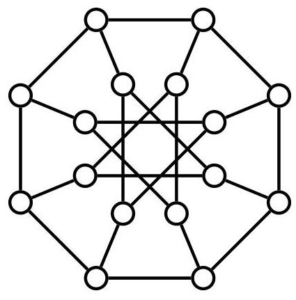
Figure 2.1: The generalised Petersen graph $\mathrm{G}(8,3)$.

Chapter 3

Graphs on groupoids

In this Chapter, we present how graphs are defined on algebraic structures, most notably, groupoids. Furthermore, we present meta-Cayley graphs. The class of graphs which we will introduce in the next chapter will be of this type.

3.1 Cayley graphs

Graphs can be defined on various algebraic structures. Most commonly, graphs are defined on groups. In doing so, the vertices of the graph are naturally defined as the elements of the group. In order to define the irreflexive and symmetric relation, so that Definition 2.1 is satisfied, subsets of the group elements are chosen which satisfy certain conditions. These subsets are known as Cayley sets and are defined as follows.

Definition 3.1. Let $G$ be a group and let $1_{G}$ be the identity element of $G$. Let $S \subset G$. If
(i) $1_{G} \notin S$ and
(ii) $s \in S$ implies $s^{-1} \in S$,
then $S$ is called a Cayley set on $G$.

Now let $G$ be a group and $S$ a Cayley set on $G$. We define a relation $E$ on $G$ by $(x, y) \in E$ if and only if $y=x s$ where $s \in S$. We then have $y s^{-1}=x$ so that $(y, x) \in E$ since $s^{-1} \in S$. Therefore $E$ is symmetric. Also, since $1_{G} \notin S$ it is impossible that $x=x s$ for some $s \in S$. Therefore $(x, x) \notin E$ and $E$ is irreflexive. This brings us to the following definition of a Cayley graph.

Definition 3.2. Let $G$ be a group and $S$ a Cayley set on $G$. The graph $\Gamma$ consisting of the vertex set

$$V(\Gamma)=G$$

and edge set

$$E(\Gamma)=\{[x, x s]: x \in G, s \in S\}$$

is called a Cayley graph on $G$ and is denoted as $\operatorname{Cay}(G, S)$.
Example 3.3. Consider the symmetric group $S_{3} . \quad U=\{(12),(123),(132)\}$ is a Cayley set on $S_{3}$ since it is closed under inverses and does not contain the identity element. The Cayley graph $\operatorname{Cay}\left(S_{3}, U\right)$ is below.

It is easy to verify that the edges drawn above correspond exactly to the set $E=$ $\left\{[x, x s]: x \in S_{3}, s \in U\right\}$.

In Gauyacq [5] the notion of Cayley graphs on groups was generalised to loop structures and in [13] it was generalised to groupoids. In [13] it was in fact shown

that every graph can be represented as a Cayley graph on a groupoid. This brings us to the following definitions.

Definition 3.4. Let $A$ be a groupoid and let $S \subset A$. If
(i) $a \notin a S$ for any $a \in A$ and
(ii) $a \in(a s) S$ for any $a \in A$ and $s \in S$,
then $S$ is called a Cayley set on $A$.
We note that if $A$ is a group then the conditions in Definition 3.4 coincide with the conditions in Definition 3.1.

Now let $A$ be a groupoid and $S$ a Cayley set on $A$. Let us verify the required irreflexive and symmetric relation $E$. Just as with groups, we define $E$ on $A$ by $(x, y) \in E$ if and only if $y=x s$ where $s \in S$. If $(x, y) \in E$ then $y=x s$ for some $s \in S$, and we also have that $x=(x s) s^{\prime}$ for some $s^{\prime} \in S$. Therefore $y s^{\prime}=(x s) s^{\prime}=x$ so that $(y, x) \in E$ and $E$ is symmetric. It is also clear that $E$ is irreflexive since $x \notin x S$.

Naturally, Cayley graphs on groupoids are defined exactly as Cayley graphs on groups. Formally it is as follows.

UNIVERSITY of the
Definition 3.5. Let $A$ be a groupoid and $S$ a Cayley set on $A$. The graph $\Gamma$ consisting of the vertex set

$$V(\Gamma)=A$$

and edge set

$$E(\Gamma)=\{[a, a s]: a \in A, s \in S\}$$

is called a Cayley graph on $A$ and is denoted as $\operatorname{Cay}(A, S)$.
In the literature, it is generally not explicitly stated that a Cayley graph is Cayley on a group. If a graph is refered to as Cayley, it is assumed to mean Cayley on a group. However, since we will be dealing with Cayley graphs on loops, we will be explicit in refering to Cayley graphs on groups.

3.2 Quasi-associativity

As alluded to previously, graphs which are Cayley on a group have been proven to be vertex-transitive, but the reverse implication does not hold. However, it has been shown that for a Cayley graph on a groupoid $\operatorname{Cay}(A, S)$, all the structure that is required for vertex-transitivity is that $A$ is a quasi-group and $S$ conforms to a certain type of weak associativity called quasi-associativity. This notion of quasi-associative subsets was first introduced by Gauyacq in [5] who termed them right associative. As elsewhere $[13,14,15,16]$, we will continue to call them quasi-associative.

Definition 3.6. Let $A$ be a groupoid and $S$ a subset of $A$. If for all $x, y \in A$ we have that

$$x(y S)=(x y) S$$

then $S$ is called a quasi-associative subset of $A$.
Proposition 3.7. [15] Let $A$ be a quasi-group and $S$ a quasi-associative Cayley set on $A$. Then the graph $\Gamma=\operatorname{Cay}(A, S)$ is vertex-transitive.

Proof. For each $a \in A$ we denote by $\lambda_{a} \in A \longrightarrow A$ the left translation

$$\lambda_{a}(x)=a x$$

for any $x \in A$. Since $A$ is a quasi-group, each $a x$ is unique in $A$ for a given $a \in A$ and any $x \in A$. Therefore, $\lambda_{a}$ is a permutation of $V(\Gamma)$.

Every edge in $\Gamma$ is of the form $[x, x s]$ for some $x \in A$ and some $s \in S$. Taking $\lambda_{a}$ of $[x, x s]$ we get

$$\lambda_{a}([x, x s])=\left[\lambda_{a}(x), \lambda_{a}(x s)\right]=[a x, a(x s)]=\left[a x,(a x) s^{\prime}\right]$$

for some $s^{\prime} \in S$. Thus $\lambda_{a}$ is edge-preserving and $\lambda_{a} \in \operatorname{Aut} \operatorname{Cay}(A, S)$.
Now let $x, y \in V(\Gamma)$. Since $A$ admits left cancellation, there exists a unique $a$ such that $a x=y$. Therefore, for any $x, y \in V(\Gamma)$, there exists some $\lambda_{a} \in \operatorname{Aut} \operatorname{Cay}(A, S)$ such that $\lambda_{a}(x)=y$ so that Aut $\Gamma$ acts transitively on $V(\Gamma)$. Therefore, $\Gamma=$ $\operatorname{Cay}(A, S)$ is vertex-transitive.

Remark 3.8. If $A$ is a group then the set of left translations forms a group under composition. This is an application of Cayley’s theorem. The set of left translations

has the same order as the set of vertices. Thus if $A$ is a group, then the set of left translations acts regularly on the set of vertices.

Graphs which can be represented by a quasi-group and a quasi-associative Cayley set are called quasi-Cayley graphs.

The following is an example of a graph defined on a groupoid, which in fact turns out to be a loop, with a quasi-associative Cayley set.

Example 3.9. [15] Let $n$ and $r$ be integers such that $(n, r)=1$ with $r^{2} \equiv \pm 1$ $(\bmod n)$. Consider the set $M(n, r)=\mathbb{Z}_{2} \times \mathbb{Z}_{n}$ paired with the binary operation defined by $(x, y)\left(x^{\prime}, y^{\prime}\right)=\left(x+x^{\prime}, y+r^{x} y^{\prime}\right)$ where $r$ is read as modulo $n$. It is clear that $(0,0)$ is the identity of $M(n, r)$. Suppose that $(x, y)\left(x^{\prime}, y^{\prime}\right)=(x, y)\left(x^{\prime \prime}, y^{\prime \prime}\right)$. This implies that

$$\begin{aligned} & \left(x+x^{\prime}, y+r^{x} y^{\prime}\right)=\left(x+x^{\prime \prime}, y+r^{x} y^{\prime \prime}\right) \\ & \Rightarrow x+x^{\prime}=x+x^{\prime \prime} \text { and } y+r^{x} y^{\prime}=y+r^{x} y^{\prime \prime} \\ & \Rightarrow x^{\prime}=x^{\prime \prime} \text { and } r^{x} y^{\prime}=r^{x} y^{\prime \prime} \\ & \Rightarrow\left(x^{\prime}, y^{\prime}\right)=\left(x^{\prime \prime}, y^{\prime \prime}\right) \end{aligned}$$

Suppose also that $\left(x^{\prime}, y^{\prime}\right)(x, y)=\left(x^{\prime \prime}, y^{\prime \prime}\right)(x, y)$. This implies that

$$\begin{aligned} & \left(x^{\prime}+x, y^{\prime}+r^{x^{\prime}} y\right)=\left(x^{\prime \prime}+x, y^{\prime \prime}+r^{x^{\prime \prime}} y\right) \\ & \Rightarrow x^{\prime}+x=x^{\prime \prime}+x \text { and } y^{\prime}+r^{x^{\prime}} y=y^{\prime \prime}+r^{x^{\prime \prime}} y \\ & \Rightarrow x^{\prime}=x^{\prime \prime} \text { and } y^{\prime}=y^{\prime \prime} \\ & \Rightarrow\left(x^{\prime}, y^{\prime}\right)=\left(x^{\prime \prime}, y^{\prime \prime}\right) \end{aligned}$$

Therefore, $M(n, r)=\mathbb{Z}_{2} \times \mathbb{Z}_{n}$ is a loop.
Consider the set $S=\{(0,1),(0,-1),(1,0)\} \subset M(n, r)$. For any $(x, y) \in M(n, r)$ we have $(x, y) S=\left\{\left(x, y+r^{x}\right),\left(x, y-r^{x}\right),(x+1, y)\right\}$ so that $(x, y) s \neq(x, y)$ for any $s \in S$. We also have that

$$\begin{aligned} ((x, y)(0,1))(0,-1) & =(x, y) \\ ((x, y)(0,-1))(0,1) & =(x, y), \text { and } \\ ((x, y)(1,0))(1,0) & =(x, y) \end{aligned}$$

so that $(x, y) \in((x, y) s) S$ for any $s \in S$. Therefore $S$ is a Cayley set on $M(n, r)$.

For any $(x, y),\left(x^{\prime}, y^{\prime}\right) \in M(n, r)$ we have

$$\begin{aligned} & \left((x, y)\left(x^{\prime}, y^{\prime}\right)\right) S \\ & =\left\{\left(x+x^{\prime}, y+r^{x} y^{\prime}\right)(0,1),\left(x+x^{\prime}, y+r^{x} y^{\prime}\right)(0,-1),\left(x+x^{\prime}, y+r^{x} y^{\prime}\right)(1,0)\right\} \\ & =\left\{\left(x+x^{\prime}, y+r^{x} y^{\prime}+r^{x+x^{\prime}}\right),\left(x+x^{\prime}, y+r^{x} y^{\prime}-r^{x+x^{\prime}}\right),\left(x+x^{\prime}+1, y+r^{x} y^{\prime}\right)\right\} \end{aligned}$$

and

$$\begin{aligned} & (x, y)\left(\left(x^{\prime}, y^{\prime}\right) S\right) \\ & =\left\{(x, y)\left(\left(x^{\prime}, y^{\prime}\right)(0,1)\right),(x, y)\left(\left(x^{\prime}, y^{\prime}\right)(0,-1)\right),(x, y)\left(\left(x^{\prime}, y^{\prime}\right)(1,0)\right)\right\} \\ & =\left\{(x, y)\left(x^{\prime}, y^{\prime}+r^{x^{\prime}}\right),(x, y)\left(x^{\prime}, y^{\prime}-r^{x^{\prime}}\right),(x, y)\left(x^{\prime}+1, y^{\prime}\right)\right\} \\ & =\left\{\left(x+x^{\prime}, y+r^{x}\left(y^{\prime}+r^{x^{\prime}}\right)\right),\left(x+x^{\prime}, y+r^{x}\left(y^{\prime}-r^{x^{\prime}}\right)\right),\left(x+x^{\prime}+1, y+r^{x} y^{\prime}\right)\right\} \\ & =\left\{\left(x+x^{\prime}, y+r^{x} y^{\prime}+r^{x} r^{x^{\prime}}\right),\left(x+x^{\prime}, y+r^{x} y^{\prime}-r^{x} r^{x^{\prime}}\right),\left(x+x^{\prime}+1, y+r^{x} y^{\prime}\right)\right\} \end{aligned}$$

so that $S$ is quasi-associative if $\left\{r^{x} r^{x^{\prime}},-r^{x} r^{x^{\prime}}\right\}=\left\{r^{x+x^{\prime}},-r^{x+x^{\prime}}\right\}$, which is true since $r^{2} \equiv \pm 1$.

The graph $\operatorname{Cay}(M(n, r), S)$ is defined on a loop with a quasi-associative Cayley set so that it is quasi-Cayley and vertex-transitive.

As it turns out, the class of graphs referred to in Example 3.9 is in fact isomorphic to the generalised Petersen graphs.

WESTERN CAPE

Proposition 3.10. [15] Let $M(n, r)$ and $S$ be as in Example 3.9. Then $\operatorname{Cay}(M(n, r)$, $S) \cong G(n, r)$.

Proof. Define a mapping $\phi: V(G(n, r)) \longrightarrow V(\operatorname{Cay}(M(n, r), S))$ by

$$v_{i} \mapsto(0, i) \text { and } u_{i} \mapsto(1, i)$$

Clearly $\phi$ is a bijection.
We also have the following

$$\begin{aligned} \phi\left(\left[v_{i}, v_{i+1}\right]\right) & =[((0, i),(0, i+1)] \\ & =[(0, i),(0, i)(0,1)] \\ \phi\left(\left[u_{i}, u_{i+r}\right]\right) & =[((1, i),(1, i+r)] \\ & =[(1, i),(1, i)(0,1)] \end{aligned}$$

$$\begin{aligned} \phi\left(\left[v_{i}, u_{i}\right]\right) & =[((0, i),(1, i)] \\ & =[(0, i),(0, i)(1,0)] \end{aligned}$$

so that $\phi$ is a bijective homomorphism.
It is clear that $|E(\operatorname{Cay}(M(n, r), S))|=|E(G(n, r))|$ since both graphs have the same degree. Therefore, by Lemma $2.5 \phi$ is an isomorphism.

As mentioned previously, every graph is a Cayley graph on some groupoid. In [14] it was shown that every vertex-transitive graph is a Cayley graph on a left loop with respect to a quasi-associative Cayley set. In view of this, the determination of VTNCGs translates to finding Cayley graphs on left loops with respect to quasiassociative Cayley sets which cannot be represented as Cayley graphs on groups. For our purposes, we then desire to find a suitable loop on which we can construct our vertex-transitive graphs.

3.3 Meta-Cayley graphs

Alspach and Parsons introduced a class of vertex-transitive graphs called metacirculant graphs in [2]. This class of graphs contains many VTNCGs. They are defined on the direct product of two cyclic groups, with the definition of edges involving some interaction between the groups which resembles the twisting used in defining semi-direct products of groups. These graphs were first shown to be quasi-Cayley by Gauyacq in [5]. In [16] they were generalised from cyclic groups to general groups.

It is a well-known result that if the twisting map in the semi-direct product of groups is a group homomorphism, then the semi-direct product is a group itself. For the semi-direct product to be a loop, much less structure is required for the twisting map. Left and right cancellability are maintained without any condition on the twisting map. For the existence of an identity element the twisting map need only satisfy a weak condition. That is, that the twisting map maps the identity element in the first group to the identity map of the second group. In the generalisation of metacirculant graphs from cyclic groups to general groups, only this key characteristic of the twisting map was maintained. The resultant graphs of this generalised construction are called meta-Cayley graphs. Meta-Cayley graphs will be suitable for our purposes.

Before we can present the definition of meta-Cayley graphs, it is necessary for us to first present some propositions and lemmas. The following proposition shows that the semi-direct product of two groups with a twisting map that satisfies the weak condition mentioned previously is indeed a loop.

Proposition 3.11. ([16]) Let $A$ and $A^{\prime}$ be groups. Let $Q=A \times_{f} A^{\prime}$ be the semi-direct product of $A$ and $A^{\prime}$ such that $f(e)$ is the identity map on $A^{\prime}$, where $e$ is the identity element of $A$. Then $Q$ is a loop.

Proof. Let $\left(a, a^{\prime}\right),\left(b, b^{\prime}\right) \in Q$. Since $A$ and $A^{\prime}$ are groups, there exists unique $x$ and $x^{\prime}$ such that $a x=b$ and $a^{\prime} x^{\prime}=b^{\prime}$. Also, since $f_{a}$ is an automorphism of $A^{\prime}$, there exists a unique $x^{\prime \prime}$ such that $f_{a}\left(x^{\prime \prime}\right)=x^{\prime}$. Therefore, there exists a unique $\left(x, x^{\prime \prime}\right)$ such that $\left(a, a^{\prime}\right)\left(x, x^{\prime \prime}\right)=\left(b, b^{\prime}\right)$ so that $Q$ is a left quasi-group.

Since $A$ and $A^{\prime}$ are groups, there exists unique $y$ and $y^{\prime}$ such that $y a=b$ and $y^{\prime} f_{y}\left(a^{\prime}\right)=b^{\prime}$. Therefore, there exists a unique $\left(y, y^{\prime}\right)$ such that $\left(y, y^{\prime}\right)\left(a, a^{\prime}\right)=\left(b, b^{\prime}\right)$ so that $Q$ is a right quasi-group.

Furthermore, let $e$ and $e^{\prime}$ be the identity elements of $A$ and $A^{\prime}$ respectively. Then $(x, y)\left(e, e^{\prime}\right)=\left(x e, y f_{x}\left(e^{\prime}\right)\right)=\left(x e, y e^{\prime}\right)=(x, y)$ and $\left(e, e^{\prime}\right)(x, y)=\left(e x, e^{\prime} f_{e}(y)\right)=$ $\left(e x, e^{\prime} y\right)=(x, y)$ so that $\left(e, e^{\prime}\right)$ is the identity. Therefore, $Q=A \times_{f} A^{\prime}$ is a loop.

Now that we know we can sufficiently find a loop by taking the semi-direct product of two groups as above, the crux of the matter with regards to constructing metaCayley graphs is the determination of quasi-associative Cayley sets. Before we show how we determine these meta-Cayley sets, we first need the following lemmas.

Lemma 3.12. Let $A$ be a loop and let $U_{1}, U_{2}, \ldots, U_{k}$ be quasi-associative subsets of A. Then $U:=\bigcup U_{i}$ is quasi-associative in $A$.

Proof. Let $a, b \in A$ and let $s \in U$ so that $s \in U_{i}$ for some $i$. Then $a(b s)=(a b) s^{\prime}$ where $s^{\prime} \in U_{i}$. Therefore $s^{\prime} \in U$ and $U$ is quasi-associative in $A$.

Lemma 3.13. [16] Let $A$ be a loop with an identity element $e$, and $U$ a quasiassociative subset of $A$ such that $e \notin U$. Then $U$ is Cayley if $U^{-1} \subseteq U$.

Proof. Let $U$ be a quasi-associative subset of $A$ with $e \notin U$ and $U^{-1} \subseteq U$. It is clear that $a \notin a U$ for any $a \in A$. For any $a \in A$ and $u \in U$, we have that $a=a e=a\left(u u^{-1}\right)=(a u) u^{\prime}$ for some $u^{\prime} \in U$. Therefore, $a \in(a u) U$ for any $a \in A$

and $u \in U$. Therefore, $U$ is Cayley.
Proposition 3.14. ([16]) Let $A$ and $A^{\prime}$ be groups and $Q$ be as in Proposition 3.11. For each $x \in A$, let $L_{x}$ be a (possibly empty) subset of $A^{\prime}$ such that
(a) $e^{\prime} \notin L_{e}$ where $e$ and $e^{\prime}$ are the identity elements of $A$ and $A^{\prime}$ respectively;
(b) $L_{x^{-1}}=f_{x}^{-1}\left[L_{x}^{-1}\right]$ for any $x \in A$;
© $f_{a} f_{b}\left[L_{x}\right]=f_{a b}\left[L_{x}\right]$ for any $a, b \in A$.

Let $U$ be the subset of $Q$ defined by

$$U:=\bigcup_{x \in A}\left(\{x\} \times L_{x}\right)$$

Then $U$ is a quasi-associative Cayley set on $Q$.
Proof. Since $A$ and $A^{\prime}$ are groups, both $\{x\}$ and $L_{x}$ are trivially quasi-associative in $A$ and $A^{\prime}$ respectively for all $x \in A$. Let $(a, b),\left(a^{\prime}, b^{\prime}\right) \in Q$ and $(x, s) \in\{x\} \times L_{x}$ for some $x \in A$. Then

$$\begin{aligned} (a, b)\left(\left(a^{\prime}, b^{\prime}\right)(x, s)\right) & =(a, b)\left(a^{\prime} x, b^{\prime} f_{a^{\prime}}(s)\right) \\ & =\left(a a^{\prime} x, b f_{a}\left(b^{\prime} f_{a^{\prime}}(s)\right)\right) \\ \text { WEST } & =\left(a a^{\prime} x, b f_{a}\left(b^{\prime}\right) f_{a}\left(f_{a^{\prime}}(s)\right)\right) \\ & =\left(a a^{\prime} x, b f_{a}\left(b^{\prime}\right) f_{a a^{\prime}}\left(s^{\prime}\right)\right) \\ & =\left(a a^{\prime}, b f_{a}\left(b^{\prime}\right)\right)\left(x, s^{\prime}\right) \\ & =\left((a, b)\left(a^{\prime}, b^{\prime}\right)\right)\left(x, s^{\prime}\right) \end{aligned}$$

for some $\left(x, s^{\prime}\right) \in\{x\} \times L_{x}$. Therefore, $\{x\} \times L_{x}$ is quasi-associative in $Q$. By Lemma $3.12, U$ is quasi-associative in $Q$.

Clearly, $\left(e, e^{\prime}\right) \notin U$. In view of Lemma 3.13, it is enough to show that $U^{-1} \subseteq U$. For each $x \in A$, consider the set $U_{x}=\left(\{x\} \times L_{x}\right) \cup\left(\left\{x^{-1}\right\} \times L_{x^{-1}}\right)$. We have

$$\left(\{x\} \times L_{x}\right)^{-1}=\left(\left\{x^{-1}\right\} \times f_{x}^{-1}\left[L_{x}^{-1}\right]\right)=\left(\left\{x^{-1}\right\} \times L_{x^{-1}}\right)$$

and

$$\left(\left\{x^{-1}\right\} \times L_{x^{-1}}\right)^{-1}=\left(\{x\} \times f_{x^{-1}}^{-1}\left[L_{x^{-1}}^{-1}\right]\right)=\left(\{x\} \times L_{x}\right)$$

Hence $U_{x}=U_{x}^{-1}$ for any $x \in A$. It is also easy to see that

$$\bigcup_{x \in A} U_{x}=U$$

Therefore $U=U^{-1}$ and by Lemma 3.13, $U$ is Cayley.

With $Q$ and $U$ as above, the resultant graph $\operatorname{Cay}(Q, U)$ is then necessarily vertextransitive. This brings us to the definition of meta-Cayley graphs.

Definition 3.15. Let $A$ and $A^{\prime}$ be groups. Let $Q=A \times_{f} A^{\prime}$ be the semi-direct product of $A$ and $A^{\prime}$ such that $f(e)$ is the identity map on $A^{\prime}$, where $e$ is the identity element of $A$. For each $x \in A$, let $L_{x}$ be a (possibly empty) subset of $A^{\prime}$ such that
(a) $e^{\prime} \notin L_{e}$ where $e$ and $e^{\prime}$ are the identity elements of $A$ and $A^{\prime}$ respectively;
(b) $L_{x^{-1}}=f_{x}^{-1}\left[L_{x}^{-1}\right]$ for any $x \in A$;
© $f_{a} f_{b}\left[L_{x}\right]=f_{a b}\left[L_{x}\right]$ for any $a, b \in A$.

Let $U$ be the subset of $Q$ defined by

$$U \cong \bigcup\left(\{x\} \times L_{x}\right)$$