Credit Risk: Implementing Structural Models

Credit Risk: Implementing Structural Models

Victor Olofi Omomehin (victor.o.omomehin@aims-senegal.org)
African Institute for Mathematical Sciences (AIMS), Senegal
Supervised by: Prof. Tom Carroll
University College Cork, Cork, Ireland

October 6, 2022
Submitted in partial fulfilment of the requirements for the award of Master of Science in Mathematical Sciences at AIMS Senegal

DECLARATION

This work was carried out at AIMS Senegal in partial fulfilment of the requirements for a Master of Science Degree.

I hereby declare that except where due acknowledgement is made, this work has never been presented wholly or in part for the award of a degree at AIMS Senegal or any other University.

Student: Victor Olofi Omomehin

ACKNOWLEDGEMENTS

To Almighty God belongs the glory, thanks and praises.
I would like to express my sincere gratitude to my supervisor, Prof. Tom Carroll, who taught me Computational Finance with Python and introduced me to the field of Credit Risk. I immensely appreciate the time and efforts he directed toward the progress of my research. His guidance was crucial to the development of this thesis, which would not have been the same without our weekly meeting discussions. A very big thanks goes to my tutor, Dr. Mouhamad M. Allaya for sharing some of his textbooks and organizing our weekly meetings on Skype.

I would also like to thank the African Institute for Mathematical Sciences (AIMS-Senegal) for providing me with this scholarship and the opportunity to study alongside other bright-minded fellow students from neighboring African countries. To my entire classmates (AIMS 2019-2021), I wish you all the best in your endeavors.

Finally, I thank my mother and my siblings for their constant support and countless sacrifices. Without them, I could never accomplish so much and reach this milestone in my life.

DEDICATION

To the memory of my father, Mr Omomehin Abayomi.

Abstract

Over the years creditors suffer losses due to failure on the part of borrowers to meet debt obligations. It has become imperative to recognize and develop credit risk techniques to mitigate the financial risks involved in lending. Lenders and investors access credit risk of individuals, corporations, or government through credit risk modeling. In this thesis, we studied three major structural credit risk models namely, the Merton, the Black and Cox, and the KMV model. In our analysis, we utilized the Merton Model to analyze Apple company data. The analysis includes: Computing the default probability of the company coupled with the estimation of the company’s asset market value through the use of the Iterative procedure. Furthermore, we investigate the relationship between the “actual” and “risk-neutral” probability of default. Our research findings show that the risk-neutral probability of default serves as upper bound for the actual probability of default.

Keywords: Credit risk, Merton model, Black and Cox model, KMV model, Actual default probability (ADP), Risk-neutral default probability (RNDP), Expected default frequency (EDF), Iterative procedure, Non-linear equations system, Capital Asset Pricing model (CAPM).

Contents

Declaration … i
Acknowledgements … ii
Dedication … iii
Abstract … iv
1 Introduction … 1
1.1 Aims and Objectives … 1
1.2 What is Credit Risk … 2
1.2.1 Credit Spread … 2
1.2.2 Credit Rating … 3
1.2.3 Credit Default Swap (CDS) … 4
1.2.4 Factors affecting credit risk: … 4
1.2.5 Qualitative Credit Risk Models: … 5
1.2.6 Quantitative Credit Risk Models: … 5
1.3 Structural Credit Risk Models: … 5
1.4 Reduced-form Credit Risk Model: … 6
1.5 Glossary … 6
2 Literature Review … 7
2.1 Drawbacks and Extensions … 8
3 Methodology … 10
3.1 Merton Model: … 10
3.1.1 Black-Scholes Option Pricing Framework … 11
3.1.2 Modeling the Actual Probability of Default (APD) … 13
3.1.3 Risk Neutral Probability of Default … 15
3.1.4 Credit spread implied by the Merton model … 15

3.1.5 Estimating Asset Value $\left(A_{i}\right)$ and Volatility $\left(\sigma_{A}\right)$ … 16
3.1.6 Nonlinear system of equations approach … 16
3.1.7 Derivation of Asset and Equity Volatility Relation … 16
3.2 Black and Cox Model … 19
3.2.1 Default Barrier … 19
3.2.2 Probability of Default … 19
3.2.3 Survival Probability … 20
3.3 Moody KMV model … 21
3.3.1 Shifting from Merton Framework to KMV … 21
3.3.2 Default Point (DP) … 21
3.3.3 Distance to Default (DD) … 22
3.3.4 Expected Default Frequency (EDF) … 22
3.3.5 Estimating Asset Value $\left(A_{i}\right)$ and Volatility $\left(\sigma_{A}\right)$ … 24
3.3.6 Iterative Approach … 25
4 Data Analysis … 26
4.1 Data Description … 26
4.2 Data Implementation … 26
4.2.1 Iterative Procedure … 26
4.2.2 Capital Asset Pricing Model (CAPM) … 27
4.3 Results and Discussions … 28
4.3.1 Asset iterates (Market value) … 29
4.3.2 Annualized volatility … 30
4.3.3 Drift rate … 30
4.3.4 Actual Probability of Default (APD) … 31
4.3.5 Risk-Neutral Versus Actual Default Probability … 32
5 Conclusion … 34
6 Appendix … 35
References … 39

1. Introduction

The term “Credit” goes way back to ancient civilizations where creditors pay less attention to credit risk. Default in one party (the debtor) often leads to quarrels and this breaks existing relationships among families, kinsmen, friends, etc. In a bid to resolve this problem, many measures were put in place, one of those was the one found in Hammurabi’s Code of law. Hammurabi the Babylonian king who lived 4000 years ago wrote this code and outlined the basic rule for borrowing. The code described failure to pay a debt as a crime and should be treated in the same way as theft and fraud. The penalties for defaulting may include debtors being sold in debt slavery while the debtor’s spouse and children would be forced into slavery (three-year term of slavery). However, the code didn’t address concepts such as interest and collateral. These concepts were spotted in some ancient religious books like the Bible and the Quran where stern restrictions were issued to followers regarding how much interest to be charged on a loan.

During the Middle Ages, laws were also made specifically to deal with debtors. The law allows creditors to drag debtors to court to obtain judgment against the debtor. This often resulted in court seizing valuable things from the debtor’s home. Sometimes the debtor would be sent to debtor’s jail until the debtor’s family could pay off the debt or until the creditor forgave it. For the most part at various places and times in ancient history, credit default was a crime and it was punishable by death, mutilation, torture, imprisonment, or enslavement and sometimes punishments could also be extended to debtor’s dependents. For example, unpaid debts could sometimes be transferred to relatives or political entities. Considering the potential consequences, one may ask why would anyone borrow or lend money during ancient times. Borrowers risked horrendous consequences from default, while lenders faced legal obstacles to collecting money owed. Coming to the modern world, there have always been various financial risks faced by financial institutions, banks, and other subjects. Various financial crises that have been experienced in the past or recent times have shown how important it is to properly predict, estimate and recognize risks. Risk management and prediction of potential losses are crucial factors in order to maintain sustainability of business activities of institutions.

1.1 Aims and Objectives

The aims and objectives of this thesis are clear and stated as follows:

1. To understand credit risk from a practical point of view.
2. To study various credit risk models with their assumptions.
3. To implement the Merton model on Apple company’s stock data (AAPL).
4. To evaluate the unobserved market value of the firm’s assets using the Iterative procedure.
5. To model probability of default associated to a risky and non-risky asset.
6. To examine the relationship between the actual and the risk-neutral default probability.

1.2 What is Credit Risk

Credit risk is a measure of the creditworthiness of a borrower. In calculating credit risk, lenders are gauging the likelihood they will recover all of their principal and interest. In other words, lenders are judging borrowers’ ability to pay back debt when making a loan. Credit risk models depend on many complex factors, thus the need to develop sophisticated credit risk rating models. Over the years many credit risk models have been created in an attempt to measure the risk in lending. These models fall into two broad categories, qualitative and quantitative. Before going into qualitative and quantitative models, let’s first talk about some important terms in credit risk such as Credit Spread, Credit Rating and Credit Default Swap.

1.2.1 Credit Spread

Credit spread can be defined in terms of a bond or option pricing. In the bond market, credit spread is called yield spread and refers to the difference between two bonds’ yields that are the same in all respects except their credit rating. The credit spread is a means of comparing the creditworthiness of different borrowers in the capital markets. Credit spread in option pricing is considered as a strategy constructed by selling an option and buying another option in the same class at different strike prices with the same expiration.

Figure 1.1: Credit spread in option

1.2.2 Credit Rating

Credit rating simply determines the likelihood that the borrower will pay back a loan without defaulting. Credit rating and Credit score are often used interchangeably in some cases but yet are distinct. Credit score is assigned to an individual, and the score is a numeric value ranging from 300 to 850 . Credits ratings on the other hand are expressed in letter grade and they are assigned to government and businesses. Letter grade can be investment grade (good rating) or speculative grade (bad rating). Investment Grade represents high likelihood to meet payment obligations while speculative grade indicates high risk of default. The table below presents types of credit rating grade.

Figure 1.2: Credit Rating Scale

Image source : http://ctstatefinance.org/bonding/bondratings

1.2.3 Credit Default Swap (CDS)

A credit default swap is a financial derivative or some kind of insurance contract that allows the transfer of credit risk from one party to another. In a CDS, one party “sells” risk and the counter party “buys” the risks. The buyers of CDS are provided with protection against a specific risk and in return the buyer has to agree to pay a periodic fee to the seller. On the other hand, the seller of the CDS who has now taken the transferred risk of the buyer has to pay a certain promised amount if a default should occur. For example, let’s assume that a bank grants a loan to a firm and the bank isn’t sure if the firm will be able to repay the loan. The bank decides to buy a CDS from a CDS seller in exchange for a protection which comes with compensation in the event that the firm in question should default on their loan. This protection comes at a price in which the buyer has to make series of payment to the CDS seller for accepting the transferred risk of the firm who may default in the future.

1.2.4 Factors affecting credit risk:

Credit risk is affected by several factors such as the followings

- Default probability (PD):

This refers to the likelihood that a borrower will default on their loans over a particular horizon and is obviously the most important part of a credit risk model. For individuals, this score is based on their existing credit score and their debt-income ratio. For institutions that issue bonds, this probability is determined by rating agencies like Moody’s and Standard & Poor’s. The PD generally determines the interest rate and the amount of down payment needed (collateral).

- Loss Given Default (LGD):

This refers to the total loss that the lender will suffer if the debt is not repaid. This is a critical component in credit risk modeling. For instance, imagine two borrowers with same credit scores and same debt-to-income ratios. The first borrower takes a $\$ 2,000$ loan, and the second borrows $\$ 200,000$. Even if the second individual has 100 times the income of the first, their loan represents a greater risk. This is because the lender stands to lose a lot more money in the event of default on a $\$ 200,000$ loan. Most lenders do not calculate LGD for each separate loan; instead, they review an entire portfolio of loans and estimate total exposure to loss. Several factors can influence LGD, including any collateral on the loan and the legal ability to pursue the defaulted funds through bankruptcy proceedings.

- Exposure at Default (EAD):

In the event of a default, how large will the outstanding obligation be when the default occurs? EDA answers this question by measuring total exposure that a lender is exposed to at any given point of time. It is calculated by multiplying each loan by a certain percentage depending on the particulars of the loan.

- Recovery Rate:

In the event of a default, the fraction of the exposure may be recovered through bankruptcy proceedings or some other form of settlement.

1.2.5 Qualitative Credit Risk Models:

These were the earliest or first models used and involve getting information by asking lot of questions before lending out money. Such models take into account certain factors such as debt’s seniority, collaterals, nature of business, credit history, economic indicator (inflation) etc. However, this model is subjective and depends on the lender’s personal judgment or experience about whether a specific outcome is likely to occur. It does not involve any formal calculation. The impact of subjectivity on this model led to the practice of “quantifying the qualitative” a necessary step.

1.2.6 Quantitative Credit Risk Models:

The intuition behind quantitative credit risk models is to be able to assign some kind of credit measure or comparable numbers to the likelihood of default risk. This allows lenders to make decisions based on a chosen threshold whether this is the risk they would want to hold, transfer or what interest rate to charge depending on default probability (low credit risk borrowers are charged low interest rates). The main objective of these models is to provide ways to price and to hedge financial contracts that are sensitive to credit risk. There are about five main types of credit risk quantitative models: credit scoring models, structural models, reduced-form models, credit migration models and credit portfolio models. However, in order to model the default process and recovery rates two competing methodologies emerged, namely, the structural approach and the reduced-form approach.

1.3 Structural Credit Risk Models:

Structural approaches are concerned with modeling and pricing credit risk that is specific to a particular corporate obligor (a firm). The basic idea is that a company (with limited liability) will default if the value of its assets is sufficiently low when compared to its liabilities. These models require strong assumptions on the dynamics of the firm’s assets, its debt and how its capital is structured meaning the probability of default for a firm is calculated based on the value of the firm’s assets, equity and liabilities. The main advantage of structural models is that they provide an intuitive picture, as well as an endogenous explanation for default. In other words, the structural approach aims to provide an explicit relationship between default risk and capital structure. The Merton model was the first structural model and has served as the cornerstone for all other structural models such as the Black and Cox (1976) model with a flat barrier, the Longstaff and Schwartz (1995) model with stochastic interest rates, the Collin-Dufresne and

Goldstein (2001) model with a stationary leverage, and the double exponential jump diffusion model used in Huang and Huang (2003).

1.4 Reduced-form Credit Risk Model:

In this approach, the value of the firm’s assets and its capital structure are not modeled at all, and the credit events are specified in terms of some exogenously specified jump process (as a rule, the recovery rates at default are also given exogenously). We can distinguish between the reducedform models that are only concerned with modeling of the default time called the intensity based models, and the reduced-form models with migrations between credit rating classes, called the credit migration models.

The main emphasis in the intensity-based approach is placed on modeling of random time of default, as well as evaluating conditional expectations under risk-neutral probability functionals of the default time and the corresponding cash flows. Typically, the random default time is defined as the jump time of some one-jump process. A pivotal role in evaluating the respective conditional expectations is played by the so-called default intensity process. Modeling of the intensity process, which is also known as the hazard rate process, is the starting point in the intensity approach.

1.5 Glossary

• Credit Event: a default, bankruptcy, or other situation which is recognized as affecting the creditworthiness of a country or organization and which may trigger insurance payments as defined in a credit default swap.
• Seniority: refers to the order of repayment in the event of a sale or bankruptcy of the issuer.
• Collateral: This refers to the assets owned by a borrower that can be used to secure a loan. The more collateral a borrower has, the lower the possible credit risk for a lender.
• Liquidation: is the method of putting an end to business and performing asset distribution to those claiming any money from the company.
• Sovereign risk: is the risk of a government or central bank being unwilling or unable to meet its contractual obligations.
• Debt-to-income ratio: This compares the amount a person makes against their living expenses and debt payments. Lenders use it to decide if a borrower can afford to take on a new debt payment.

2. Literature Review

The insight from the work of (Black and Scholes, 1973) and (Merton, 1974) shed more light on credit pricing models and led to the birth of structural models. (Merton, 1974) being the first of this kind paved the way for other structural models. (Jones et al., 1984) show how structural models systematically underestimated observed spreads. Their research was carried out on a sample of firms with simple capital structures observed during the year 1977 to 1981. (Ogden, 1987) confirmed this result by showing that the Merton model underpredicted spreads over U.S. treasuries by an average of 104 basis points. (Delianedis and Geske, 2001) study the credit spread proportion that is explained by default risk in a set of corporate bond data, using the (Merton, 1974) and (Geske, 1977) approach. They concluded that only a small fraction of credit spreads are explained; the remainder is due to taxes, jumps, uncertainty, and market risk factors.

Moody’s KMV (Kealhofer, McQuown, and Vasicek), being a widely accepted commercial application of structural models, extended Merton’s model by combining an empirical distribution of distance-to-default with the Vasicek-Kealhofer (VK) model to generate the Expected Default Frequency (EDF) (see Crosbie and Bohn (2003), Kealhofer (2003a), Kealhofer (2003b), and Vasicek (1984)). (Bharath and Shumway, 2004) studied the accuracy of predicting default in KMV model. The authors compare the KMV model accuracy with a simpler alternative. They discovered that the implied default probabilities from credit default swaps and corporate bond yield spreads are only weakly correlated with KMV-Merton default probabilities. The authors concluded that the KMV-Merton model does not provide a sufficient statistic for default, which can be obtained using relatively naïve hazard models. (Hillegeist et al., 2004) and (Du et al., 2004) compare the KMV model to other models and find that the KMV model does not provide adequate predictive power.

First Passage models were introduced with the work of Black and Cox (1976). Black and Cox (1976) modeled the default point as a time-dependent barrier. The default-risky coupon bonds from Black and Cox is a natural extension of (Merton, 1974) with an endogenous default boundary. (Fouque et al., 2006) studied the impact of introducing stochastic volatility into the First Passage Model, their findings resulted in short-term spreads. (Bielecki and Rutkowski, 2002) generalized the Black and Cox (1976) model to study the pricing of coupon bonds, optimal capital structure, and other types of safety covenants.
(Hull et al., 2004) present an alternative approach for estimating the non-observable asset volatility. Considering the implied volatility of options on the company’s stocks, the authors propose an approach different from the variance restriction method to measure asset volatility. The method is based on the (Geske, 1979) model, which suggests that since the equity of a company can be considered as an option on the firm’s assets, an option on the firm’s stock is a compound option, and further provides a valuation formula for such a compound option. Using the (Geske, 1979) formulation, the authors present a two-equation system that can be solved with two implied volatilities, sampled from stock options. (Geske, 1977) views the liability claims as compound options. Geske assumes that the firm is given the option of issuing new equity to service debt. (Longstaff and Schwartz, 1995) incorporate stochastic interest rates into the structural model thereby creating two-factor specifications. (Leland and Toft, 1996) consider the impact

of bankruptcy cost and taxes on the performance of the structural model. They assume the firm issues a constant amount of debt continuously with fixed maturity and continuous coupon payments. (Collin-Dufresne and Goldstein, 2001) expand the Longstaff and Schwartz model by adding a stationary leverage ratio, allowing firms to move away from their target leverage ratio in the short run only. (Zhou, 1997) and (Hilberink and Rogers, 2002) worked with structural models in which the firm’s asset value incorporates a jump component. Zhou also extends (Longstaff and Schwartz, 1995) model considering a lognormal distributed jump component. (Hilberink and Rogers, 2002) opt for an extension of (Leland and Toft, 1996) using Levy processes for downward jumps in the firm’s value.

2.1 Drawbacks and Extensions

One problem with Merton’s model is the limitation of default time to the debt maturity, ruling out the possibility of early default, regardless of what happens to the value of the firm prior to the debt maturity. For instance, if the value of the company falls to a minimum level before the debt maturity but later recovered to meet the payment of the debt at maturity, default would be avoided in Merton’s approach. (Black and Cox, 1976) often referred to as the “first-pass-time model” was developed to fix the problem of “default at maturity” in Merton’s model. The model was based on the fact that default may occur not only at maturity, but also before maturity, as long as the asset value of the firm falls below the “pre-specified barrier” which is the default trigger value. This allows defaults to occur throughout the lifetime of the reference debt or entity. Also, there were some parameters in the Merton model that were assumed to be constant. (Longstaff, 1995) improve this shortcoming of Merton’s model by presenting the short-term risk-free interest rate as a stochastic process that converges to a risk-free long-term interest rate and is negatively correlated to the asset value process, so that the immediate impact of monetary policy on the macro economy is considered.

Another disadvantage of Merton’s model is that a firm’s usual capital structure is far more complicated than a simple zero-coupon bond. Geske (1977), Geske (1979) regards the company’s debt structure as a coupon bond, where each coupon payment is considered as a compound option and a possible default cause. At each coupon payment the shareholders have the option of either making the payment to the bondholders, obtaining the right to control the company until the next coupon, or not making the payment, in which case the company defaults. Geske also extends the model to consider features such as sinking funds, safety covenants, debt subordination and limitations on payouts. Another major criticism the Merton model has received is the assumption of a constant and flat term structure of interest rates. (Jones et al., 1984) propose that “there exists evidence that introducing stochastic interest rates, as well as taxes, would improve the model’s performance.”
(Eom et al., 2003) conducted an empirical analysis of five models (Merton, Geske, Leland and Toft, Longstaff and Schwartz, as well as Collin-Dufresne and Goldstein). They assume that the asset risk premium is a stochastic process and it negatively correlated to the unexpected shock to the return of asset value. They concluded that

“Using estimates from the implementations we consider most realistic, we agree that the five structural bond pricing models do not accurately price corporate bonds. However, the difficulties are not limited to the under prediction of spreads. They all share the same problem of inaccuracy, as each has a dramatic dispersion of predicted spreads.”

3. Methodology

3.1 Merton Model:

Merton (1974), use Black and Scholes (1973) option pricing theory to model a firm’s capital structure (equity and debt) relating it to credit risk on the assumption that default will be triggered if the value of the assets fall below the value of its liabilities at maturity.

Consider a scenario:

Suppose that, at time $t, A_{t}$ is the value of the company’s assets composed of the company’s equity $E_{t}$ and debt $D_{t}$ in the form of a zero-coupon bond with a face value $L$ maturing at time $\mathrm{T}>\mathrm{t}$. The capital structure is given by the accounting equation:

$$A_{t}=E_{t}+D_{t}$$

At time $t=0$, the bond is sold at $D_{0}$ on the market. The company must pay the value of $L$ to its creditors at time $t=T$ (maturity). However, there is a possibility that the company may default on its debt obligation if the value of the company (Assets) falls below its liabilities $L$ at maturity. In this scenario the company is liquidated and the assets are distributed in order of seniority. It is assumed that debt takes precedence over equity, therefore, creditors are paid first while the leftover value of the company is reserved for the equity holders.

Figure 3.1: Equity holders and Creditors Payoff.

From Figure 3.1 we observed the following possibilities :

- Equity holders:

If $A_{T} \geq L$ then there is sufficient money to pay the liability $L$ and equity holders received what’s left in the amount of $A_{T}-L$. However, if $A_{T}<L$ then there is not enough money to pay the company’s liabilities hence the creditors keep what is left of the company while the equity holders walk away with nothing. Thus,

$$E_{T}=\max \left\{A_{T}-L, 0\right\}$$

This is the payoff from a European call option on the company’s assets $A_{T}$ with strike price $L$. Thus, the equity holders can be viewed as holding a call option on the value of the company with strike price $L$.

- Creditors:

If $A_{T} \geq L$ then the creditors receive full payment $L$. If $A_{T}<L$ then the creditors receive the full value of the company which is less than $L$. Thus, the creditor get:

$$D_{T}=\min \left(A_{T}, L\right)=L-\max \left\{L-A_{T}, 0\right\}$$

This is equivalent to risk-free zero-coupon bond with face value $L$ and a short put guaranteed on the firm’s assets.

3.1.1 Black-Scholes Option Pricing Framework

We can now adapt the firm’s capital structure and the assumptions stated from the above to fit the requirements of the Black-Scholes model. The fluctuation of asset value over time in the market is assumed to take the form of a random walk (see figure 3.2 below). For this reason we assume that the asset value follows a geometric Brownian motion process (GBM). The risk-neutral dynamics is given by the stochastic differential equation:

$$\frac{d A_{t}}{A_{t}}=r d t+\sigma_{A} d W_{t}, \quad A_{0}>0$$

where $W_{t}$ is a standard Brownian motion, $\sigma_{A}$ is the asset’s volatility, and $r$ is the risk-free rate of return. The solution to the above dynamic is achieved through Ito’s lemma:

Proof :

$$\begin{gathered} \text { Let } F_{t}=F\left(A_{t}\right)=\log A_{t} \text {. From Ito's lemma : } \\ d F_{t}=\frac{\partial F\left(A_{t}\right)}{\partial t} d t+\frac{\partial F\left(A_{t}\right)}{\partial A_{t}} d A_{t}+\frac{1}{2} \frac{\partial^{2} F\left(A_{t}\right)}{\partial A_{t}^{2}}\left(d A_{t}\right)^{2} \end{gathered}$$

$$\begin{gathered} \frac{\partial F\left(A_{t}\right)}{\partial t}=0, \frac{\partial F\left(A_{t}\right)}{\partial A_{t}}=\frac{1}{A_{t}}, \frac{\partial^{2} F\left(A_{t}\right)}{\partial A_{t}^{2}}=-\frac{1}{A_{t}^{2}} \\ d F_{t}=\frac{d A_{t}}{A_{t}}-\frac{1}{2}\left(A_{t} \sigma_{A}\right)^{2}\left(\frac{1}{A_{t}^{2}}\right) d t \end{gathered}$$

Substitute (3.1.4) into (3.1.5) we have:

$$d F_{t}=\left(r-\frac{1}{2} \sigma_{A}^{2}\right) d t+\sigma_{A} d W_{t}$$

On integrating both sides from 0 to t we obtain:

$$\log A_{t}=\log A_{0}+\left(r-\frac{1}{2} \sigma_{A}^{2}\right) t+\sigma_{A} W_{t}$$

so that,

$$A_{t}=A_{0} e^{t\left(r-\frac{1}{2} \sigma_{A}^{2}\right)+\sigma_{A} W_{t}}$$

Based on the assumption of equation (3.1.2), we can now apply the Black-Scholes formula (European call option) to compute the value of equity at time $\mathrm{t}(0 \leq t \leq T)$ given as:

$$E_{t}=A_{t} N\left(d_{1}\right)-L e^{-r(T-t)} N\left(d_{2}\right)$$

where:

$$\begin{gathered} d_{1}=\frac{\ln \left(\frac{A_{t}}{L}\right)+\left(r+\frac{\sigma_{A}^{2}}{2}\right)(T-t)}{\sigma_{A} \sqrt{T-t}} \\ d_{2}=d_{1}-\sigma_{A} \sqrt{T-t}=\frac{\ln \left(\frac{A_{t}}{L}\right)+\left(r-\frac{\sigma_{A}^{2}}{2}\right)(T-t)}{\sigma_{A} \sqrt{T-t}} \end{gathered}$$

$E_{t}=$ Theoretical value of a company’s equity
$A_{t}=$ Value of the company’s assets at time $t$
$L=$ Face value of the company’s debt
$t=$ Current time
$T=$ Maturity date of the bond (the time to maturity is $\tau=T-t$ ).
$r=$ Risk-free interest rate.
$N=$ Cumulative standard normal distribution.
$\sigma_{A}=$ Asset volatility of the firm, assumed constant

3.1.2 Modeling the Actual Probability of Default (APD)

Here we are interested in deriving the actual probability of default at maturity T. We will start with the assumption that the firm’s asset value follows a Geometric Brownian Motion :

$$\frac{d A_{t}}{A_{t}}=\mu d t+\sigma_{A} d W_{t}, \quad A_{0}>0$$

where $\mu$ is the firm’s drift rate. Figure 3.2 gives a brief overview on the necessary assumptions needed to compute the probability of default.

Figure 3.2: Probability of Default.

The probability of default is mathematically expressed as :

$$P_{d e f}=\operatorname{Prob}\left(A_{T} \leq L\right)$$

where $P_{d e f}$ is the probability that the market value of the firm’s assets will be equal or below its book value of liabilities at maturity. Assume the asset value is given as :

$$A_{t}=A_{0} e^{\left(\mu-\frac{\sigma_{A}^{2}}{d}\right) t+\sigma_{A} W_{t}}$$

$$\ln \left(A_{t}\right)=\ln \left(A_{0}\right)+\left(\mu-\frac{\sigma_{A}}{2}\right) t+\sigma_{A} W_{t}$$

The asset value $A_{t}$ is the solution to the asset dynamics in (3.1.9) obtained using Ito’s lemma. Substituting (3.1.12) into (3.1.10) we obtained the expression:

$$P_{d e f}=\operatorname{Prob}\left(\ln \left(A_{0}\right)+\left(\mu-\frac{\sigma_{A}}{2}\right) t+\sigma_{A} W_{t} \leq \ln (L)\right)$$

From the properties of Brownian motion we know that

$$\varepsilon_{t+T}=\frac{W(t+T)-W(t)}{\sqrt{T}} \text { and } \varepsilon_{t+T} \sim N(0,1)$$

Hence $W_{t}=\sqrt{t} \varepsilon$ and we can therefore rewrite (3.1.13) as follows:

$$\begin{gathered} P_{d e f}=\operatorname{Prob}\left(\ln \left(A_{0}\right)+\left(\mu-\frac{\sigma_{A}}{2}\right) t+\sigma_{A} \sqrt{t} \varepsilon \leq \ln (L)\right) \\ P_{d e f}=\operatorname{Prob}\left(-\frac{\ln \left(\frac{A_{0}}{L}\right)+\left(\mu-\frac{\sigma_{A}}{2}\right) t}{\sigma_{A} \sqrt{t}} \geq \varepsilon\right) \end{gathered}$$

Since $\varepsilon \sim N(0,1)$, the corresponding probability of default in (3.1.15) is written in terms of standard cumulative normal distribution where $A_{0}$ is the current value of the asset.

$$P_{d e f}=N\left(-\frac{\ln \left(\frac{A_{0}}{L}\right)+\left(\mu-\frac{\sigma_{A}}{2}\right) t}{\sigma_{A} \sqrt{t}}\right)$$

This can also be written as :

$$P_{d e f}=N(-d)=1-N(d)$$

where $N(d)$ is the survival function and d is the distance-to-default,

$$d=\frac{\ln \left(\frac{A_{0}}{L}\right)+\left(\mu-\frac{\sigma_{A}}{2}\right) t}{\sigma_{A} \sqrt{t}}$$

3.1.3 Risk Neutral Probability of Default

As we have seen from the above, the method used to get the probability of default $N(-d)$ does not involve Black-Scholes-Merton (BSM) option pricing theory. Yet similar to the BSM’s component $N\left(d_{2}\right)$ given below:

$$N\left(d_{2}\right)=N\left(\frac{\ln \left(\frac{A_{t}}{L}\right)+\left(r-\frac{\sigma_{A}^{2}}{2}\right)(T-t)}{\sigma_{A} \sqrt{T-t}}\right)$$

If we reverse (3.1.19) to become $N\left(-d_{2}\right)$ we can use this refinement to estimate the probability of default but this will be done under the assumption of the risk-neutral probability measure where all assets are expected to grow at a risk-free rate $(r)$. The probability of default associated to $N\left(-d_{2}\right)$ is called the risk-neutral probability of default. Furthermore, under the physical probability measure, the risk-free rate parameter $r$ would be replaced by a real or physical firm drift $(\mu)$ which implies the mean rate of return on the asset. The probability of default based on the physical firm drift $(\mu)$ is called the actual probability of default $N(-d)$. Note, the actual probability of default was derived from a simple statistical procedure as shown in (3.1.10) to (3.1.16). In summary, the key difference between the risk-neutral and the actual probability of default is that the former uses risk-free rate parameter $r$ while the later use a physical drift parameter $(\mu)$ which can be computed by compounding the expected asset return from the Capital Asset Pricing Model (CAPM).

3.1.4 Credit spread implied by the Merton model

Creditors are often exposed to default risk, they can hedge their position completely by purchasing a European put option written on the same underlying asset $A_{t}$ with strike price $L$. Such a put option will worth $L-A_{T}$ if $A_{T}<L$, and will be worth nothing if $A_{T}>L$. Combining these two positions (debt and put option), creditors will be guaranteed a payoff of L at time T , thus forming a risk-free position:

$$D_{t}+P_{t}=L e^{-r(T-t)}$$

where $P_{t}$ denotes the put option price at time $t$ and it is estimated by applying the Black-Scholes formula for a European put option:

$$P_{t}=L e^{-r(T-t)} N\left(-d_{2}\right)-A_{t} N\left(-d_{1}\right)$$

The corporate debt is a risky bond, and thus should be valued at a credit spread (risk premium). Let $s$ denote the continuously compounded credit spread, then the bond price $D_{t}$ can be written as:

$$D_{t}=L e^{-(r+s)(T-t)}$$

Putting (3.1.20), (3.1.21) and (3.1.22) together gives a closed-form formula for s:

$$s=-\frac{1}{T-t} \ln \left[N\left(d_{2}\right)-\frac{A_{t}}{L} e^{r(T-t)} N\left(-d_{1}\right)\right]$$

which allows us to solve for credit spread when asset level and return volatility $\left(A_{t}\right.$ and $\left.\sigma_{A}\right)$ are available for given $t, T, L$, and $r$.

3.1.5 Estimating Asset Value $\left(A_{t}\right)$ and Volatility $\left(\sigma_{A}\right)$

In order to compute the credit spread and the probability of default of a firm, one must first obtain the asset value and the asset volatility. Unfortunately, these values are not directly observable from the market. We can however find estimates for the firm’s asset value and its volatility using any of the following approaches:

• Iterative approach.
• Nonlinear system of equations approach.

Here we will start with the Nonlinear system of equations approach and then discuss the Iterative approach in the later section (Moody’s KMV section). These approaches require numerical implementation.

3.1.6 Nonlinear system of equations approach

The equations below are characterized by two unknown variables which are the unobserved asset value and its volatility. These equations are solved simultaneously for the value of $A_{t}$ and $\sigma_{A}$.

$$\begin{gathered} E_{t}=A_{t} N\left(d_{1}\right)-L e^{-r(T-t)} N\left(d_{2}\right) \\ \sigma_{E}=\frac{A_{t} \sigma_{A}}{E_{t}} N\left(d_{1}\right) \end{gathered}$$

We are familiar with (3.1.24) from the Black-Scholes Merton framework. The equity-asset volatility relationship in (3.1.25) was derived from asset and equity dynamics using Ito’s lemma.

3.1.7 Derivation of Asset and Equity Volatility Relation

Now, let’s derive the asset and equity relation in (3.1.25). First, we assume that the firm’s asset and equity follow a Geometric Brownian Motion expressed as the following stochastic differential equations:

$$\begin{aligned} & d A_{t}=\left(\mu_{A} A_{t}\right) d t+\left(\sigma_{A} A_{t}\right) d W_{t} \\ & d E_{t}=\left(\mu_{E} E_{t}\right) d t+\left(\sigma_{E} E_{t}\right) d W_{t} \end{aligned}$$

where
$\mu_{E}$ is the instantaneous “drift” of the equity price process.
$\sigma_{E}$ is the instantaneous equity volatility
$d W_{t}$ is a Wiener process.

Suppose the equity of the firm is a function of asset $(A)$ and time $(t)$ written as $E_{t}=F\left(A_{t}, t\right)$. Then a new dynamic can be found by applying Ito’s formula to the equity function and hence the following:

From Ito’s lemma

$$d E_{t}=d F=F_{t} d t+F_{A_{t}} d A_{t}+\frac{1}{2} F_{A_{t} A_{t}}\left(d A_{t}\right)^{2}$$

We substitute $d A_{t}$ from (3.1.26) into (3.1.28) we obtain :

$$d E_{t}=\left[F_{t}+F_{A_{t}}\left(\mu_{A} A_{t}\right)+\frac{1}{2} F_{A_{t} A_{t}}\left(\sigma_{A}^{2} A_{t}^{2}\right)\right] d t+F_{A_{t}}\left(\sigma_{A} A_{t}\right) d W_{t}$$

where $F_{t}=\frac{\partial F}{\partial t}=\frac{\partial E_{t}}{\partial t}, \quad F_{A_{t}}=\frac{\partial F}{\partial A_{t}}=\frac{\partial E_{t}}{\partial A_{t}}, \quad F_{A_{t} A_{t}}=\frac{\partial^{2} F}{\partial A_{t}^{2}}=\frac{\partial^{2} E_{t}}{\partial A_{t}^{2}}$.
Thus,

$$d E_{t}=\left[\frac{\partial E_{t}}{\partial t}+\frac{\partial E_{t}}{\partial A_{t}}\left(\mu A_{t}\right)+\frac{1}{2} \frac{\partial^{2} E_{t}}{\partial A_{t}^{2}}\left(\sigma_{A}^{2} A_{t}^{2}\right)\right] d t+\frac{\partial E_{t}}{\partial A_{t}}\left(\sigma_{A} A_{t}\right) d W_{t}$$

By comparing the coefficient of the Wiener processes $\left(d W_{t}\right)$ in (3.1.27) and (3.1.30) we found an important relation given by :

$$\sigma_{E}=\frac{\partial E_{t}}{\partial A_{t}}\left[\sigma_{A}\left(\frac{A_{t}}{E_{t}}\right)\right]=\frac{A_{t}}{E_{t}} \sigma_{A} \Delta$$

$\Delta=\frac{\partial E_{t}}{\partial A_{t}}$, where $\Delta$ is the hedge ratio, $N\left(d_{1}\right)$ from Black-Scholes.

$$\sigma_{E}=\frac{A_{t} \sigma_{A}}{E_{t}} N\left(d_{1}\right)$$

The application of this approach is easily illustrated through the following example.
Example 3.1.1. Assume the observable market capitalization of a public company is $\$ 50$ million and the calculated equity volatility of the company is 70.0 percent. Further, assume that the company has issued a single zero-coupon bond with principal of $\$ 40$ million that matures in two years and the current risk-free interest rate is 2.0 percent (for purposes of the model, a flat term structure is assumed).

We are interested in the value of the unknowns which are the unobserved value of the asset and its volatility. We solved this problem using a numerical approach via Python implementation.

Solution

import numpy as np
import scipy.stats as st
import scipy.optimize as opt
from math import exp
debt = 40000000
equity = 50000000
equity_vol = 0.7
T = 2
rate = 0.02
# Initializing asset's value and volatility
asset = equity + debt
asset_vol = round(equity_vol*(equity/asset),5)
def f(variables) :
    (asset,asset_vol) = variables
    d1 = (np.log(asset/debt)+(rate + T*(asset_vol**2)/2))/asset_vol*np.sqrt(T)
    d2 = d1-asset_vol*np.sqrt(T)
    # Equation 1
    f1 = equity - asset*st.norm.cdf(d1,0,1)+debt*exp(-rate*T)*st.norm.cdf(d2,0,1)
    # Equation 2
    f2 = equity_vol - asset_vol*(asset/equity)*st.norm.cdf(d1,0,1)
    solutions = [f1, f2]
    return solutions
# Solver
result = opt.newton(f,(asset,asset_vol))
print('Asset value = ',round(result[0],3) ,',','Volatility = ',round( result[1],3))
    Asset value = 88384003.659, Volatility = 0.396

Using the above approach we obtained the implied current value of the firm assets $A_{t}=$ $\$ 88,384,003.66$ and the implied asset volatility $\sigma_{A}=40 \%$. The Newton optimizer used here may not have yielded the best result. For instance, the Excel solver produces a better result estimating the asset’s value and its volatility as $A_{t}=\$ 87,138,636$ and $\sigma=42.2 \%$ respectively. If we get our hands dirty with little parameter tuning, the Newton method might yield best result. However, the goal of this illustration is to show how the nonlinear system of equations approach works with python.

3.2 Black and Cox Model

Black and Cox (1976) extend Merton’s model by refining the idea of “default at maturity” to “early default”. This implies that each time a firm’s asset value goes below a certain timedependent barrier $K(t)$, default is triggered. This time-dependent barrier is called the “Safety Covenant” and it provides the firm’s bondholders the right to force the firm to bankrupt if at anytime the firm’s value reaches or goes below a certain pre-specified threshold $K(t)$. Thus, the default time is given by:

$$\tau=\inf \left\{t>0: A_{t}<K(t)\right\}$$

Just as in the Merton model, this Simple First Passage model assumes that the asset value follows a geometric Brownian motion and outstanding debt with face value L at maturity T .

3.2.1 Default Barrier

For a specified time dependent barrier $K(t)$, the bondholders are always completely covered if $K(t)>L$, which is certainly unrealistic. However, the consistent definition of default becomes possible if $K_{T} \leq L$. One of many ways to specify the safety covenant is by choosing an increasing time dependent barrier:

$$K(t)=L_{0} e^{\gamma t}, \quad L_{0} \leq L e^{-\gamma T}$$

The inequality in (3.2.2) ensures that the safety covenants $K(t)$ never exceeds the discounted face value of the debt $L$.

3.2.2 Probability of Default

Under the risk neutral measure, the asset dynamic is assumed to follow a geometric Brownian motion:

$$\frac{d A_{t}}{A_{t}}=r d t+\sigma_{A} d W_{t}$$

We solved this stochastic differential equation using Ito’s lemma in order to obtain the value of the firm’s asset.

$$A_{t}=A_{0} e^{t\left(r-\frac{1}{2} \sigma_{A}^{2}\right)+\sigma_{A} W_{t}}$$

The first passage time to the default barrier can now be reduced to the first passage time for Brownian motion with drift.

$$\left\{A_{t}<K(t)\right\}=\left\{A_{0} e^{t\left(r-\frac{1}{2} \sigma_{A}^{2}\right)+\sigma_{A} W_{t}} \leq L_{0} e^{\gamma t}\right\}$$

$$\left\{A_{t}<K(t)\right\}=\left\{W_{t}+\sigma_{A}^{-1}\left(r-\frac{1}{2} \sigma_{A}^{2}-\gamma\right) t \leq \sigma_{A}^{-1} \log \left(\frac{L_{0}}{A_{0}}\right)\right\}$$

We define the risk neutral probability of default occurring before time $t \leq T$ as :

$$Q[0 \leq \tau<t]=Q\left[\min _{s \leq t}\left(\frac{A_{s}}{K(s)}\right) \leq 1\right]=Q\left[\min _{s \leq t} X_{s} \leq \sigma_{A}^{-1} \log \left(\frac{L_{0}}{A_{0}}\right)\right]$$

where $\quad X_{t}=W_{t}+m t, \quad m=\sigma_{A}^{-1}\left(r-\frac{\sigma_{A}^{2}}{2}-\gamma\right), \quad d=\sigma_{A}^{-1} \log \left(\frac{L_{0}}{A_{0}}\right)$
This is a classic problem of probability. By reflection principle (see Musiela and Rutkowski (2006) Part III APPENDIX) the solution is given as:

$$\begin{gathered} Q[0 \leq \tau<t]=1-F P(-d ;-m, t) \\ F P(d ; m, t)=N\left[\frac{d-m t}{\sqrt{t}}\right]-e^{2 m d} N\left[\frac{-d-m t}{\sqrt{t}}\right], d \geq 0 \end{gathered}$$

where $Q[0 \leq \tau<t]$ is the probability of default occurring before time $t \leq T$ and $\tau$ is the default time.

3.2.3 Survival Probability

The survival probability is given as :

$$F P(-d ;-m, t)=N\left[\frac{-d+m t}{\sqrt{t}}\right]-e^{2 m d} N\left[\frac{d+m t}{\sqrt{t}}\right]$$

This can also be written as:

$$F P(-d ;-m, t)=N(h 1)-h 3[N(h 2)]$$

where

$$\begin{gathered} h 1=\frac{-d+m t}{\sqrt{t}}=\frac{\log \left(\frac{A_{0}}{L_{0}}\right)+\left(r-\frac{\sigma_{A}^{2}}{2}-\gamma\right) t}{\sigma_{A} \sqrt{t}} \\ h 2=\frac{d+m t}{\sqrt{t}}=\frac{\log \left(\frac{L_{0}}{A_{0}}\right)+\left(r-\frac{\sigma_{A}^{2}}{2}-\gamma\right) t}{\sigma_{A} \sqrt{t}} \\ h 3=e^{2 m d}=\left(\frac{L_{0}}{A_{0}}\right)^{2 a}, \quad a=\frac{r-\frac{\sigma_{A}^{2}}{2}-\gamma}{\sigma} \end{gathered}$$

3.3 Moody KMV model

KMV was found and introduced in the late 80’s by Kealhofer, McQuown, and Vasicek. The model was acquired by Moody’s Corporation in 2002. Since the acquisition in 2002, the model has been maintained and developed on a continuous basis by Moody’s Corporation. KMV, now Moody’s KMV, is a structural model like the Merton model but with more realistic assumptions. This model tries to overcome many weaknesses seen in the Merton model by introducing new concepts like default point, multi-class liabilities, distance to default and Expected Default Frequency. We will briefly explain each of these concepts by blending it into the Merton model framework.

3.3.1 Shifting from Merton Framework to KMV

One has to modify some few assumptions in the original Merton model in order to move from the Merton framework to KMV’s. Here we outline the key points where KMV diverges from a strict structural model.

Figure 3.3: Expected Default Frequency.

3.3.2 Default Point (DP)

All liabilities in the Merton model are mapped to zero coupon bonds, this assumption is replaced with multiple class liabilities such as short term liabilities, long-term liabilities etc. In the KMV model default may occur before maturity and it is triggered whenever the asset value goes below a certain threshold called default point (DP). The default point of a firm is usually placed somewhere between the short-term debt and half the long-term debt.

$$D P=S T D+\frac{1}{2} L T D$$

The insight here is that the firm will always have to prioritize the short term debt over the long term debt. Furthermore, default does not necessarily occur when the firm’s asset value reaches the book value of their total liabilities. However, a firm will default when the difference between firm’s assets and the firm’s default point reaches zero.

3.3.3 Distance to Default (DD)

The default point is an essential ingredient for computing the distance to default (DD) in the KMV model. The DD is the number of standard deviations the asset value is away from default point and it is calculated from the given relation below:

$$D D=\frac{A_{t}-D P}{A_{t} \sigma_{A}}$$

Recall from the Merton model, the 1-year probability of default is given as $N(-d)$ where

$$d=\frac{\log \left(A_{t}\right)-\log (L)+\left(\mu-\frac{\sigma_{A}^{2}}{2}\right)}{\sigma_{A}}$$

According to empirical research, the quantity $\mu-\frac{\sigma_{A}^{2}}{2}$ is very close to zero hence negligible (see Crosbie and Bohn, 2002). We approximate (3.3.3) to the expression below :

$$\frac{\log \left(A_{t}\right)-\log (L)+\left(\mu-\frac{\sigma_{A}^{2}}{2}\right)}{\sigma_{A}} \approx \frac{\log \left(A_{t}\right)-\log (L)}{\sigma_{A}} \approx \frac{A_{t}-L}{\sigma_{A} A_{t}}$$

We then substitutes the liability L with the default point DP in KMV.

$$\begin{gathered} \frac{A_{t}-L}{\sigma_{A} A_{t}} \approx \frac{A_{t}-D P}{\sigma_{A} A_{t}} \\ D D=\frac{A_{t}-D P}{\sigma_{A} A_{t}} \end{gathered}$$

3.3.4 Expected Default Frequency (EDF)

The Expected Default Frequency is a fundamental quantity in the KMV model used for calculating the probability that a given firm will default within a year. In the Merton model, the probability of default is computed from a normal distribution and this does not conform to the true probability compared to the KMV’s EDF computed from empirical data. The figure below displays some of

the few relevant assumptions in the KMV model that differ from the Merton model.

Figure 3.4: Comparison of Assumptions

The EDF of a firm is given by:

$$E D F_{K M V}=F_{\text {emp }}(D D)=F_{\text {emp }}\left(\frac{A_{t}-D P}{\sigma_{A} A_{t}}\right)$$

We then replace the normal distribution function " $N($.$) " in the Merton model with a decreasing$ empirical function " $F_{\text {emp }}(.) "$. The figure below shows how this function works

Figure 3.5: Mapping from DD to EDF.

The function $\operatorname{Femp}($.$) maps the distance to default of a firm to the proportion of a huge historical$ database of companies that have similar DD value that have defaulted in the past. This implies that two different companies with the same DD will have the same EDF.

Example 3.3.1.

distance to default, $D D=\frac{1,200-800}{100}=4$.

Among the population of all the firms with $D D=4$ at one point in time, say 5000 firms, 20 defaulted in one year. Then

$$E D F_{1-y r}=\frac{20}{5000}=0.004=40 b p$$

Example 3.3.2. Federal Express (dollars in billions of US)

3.3.5 Estimating Asset Value $\left(A_{t}\right)$ and Volatility $\left(\sigma_{A}\right)$

We could simultaneously solve for the asset value and volatility using equity value and equity volatility as shown in the previous section. But, Crosbie and Bohn (2003) state that a simultaneous solution for these equations yields poor results. Instead we will use an iterative approach for optimum result of asset’s value and volatility.

3.3.6 Iterative Approach

We will begin this approach by rearranging the Black-Scholes formula in (3.1.8), we get:

$$A=\left[E+L e^{-r(T-t)} N\left(d_{2}\right)\right] \div N\left(d_{1}\right)$$

If we go back in time, say 260 trading days, we obtain a system of equations:

$$\begin{aligned} A_{t} & =\left(E_{t}+L_{t} e^{-r_{t}(T-t)}\left[N\left(d_{2}\right)_{t}\right]\right) \div N\left(d_{1}\right)_{t} \\ A_{t-1} & =\left(E_{t-1}+L_{t-1} e^{-r_{t-1}(T-(t-1))}\left[N\left(d_{2}\right)_{t-1}\right]\right) \div N\left(d_{1}\right)_{t-1} \\ \vdots & \\ A_{t-a} & =\left(E_{t-a}+L_{t-a} e^{-r_{t-a}(T-(t-a))}\left[N\left(d_{2}\right)_{t-a}\right]\right) \div N\left(d_{1}\right)_{t-a} \end{aligned}$$

Iteration 0 :

First, we start the procedure by initializing the asset value from the data using the accounting equation:

$$A_{t-a}=E_{t-a}+L_{t-a}, \quad a=0,1, \ldots, 260$$

where $L_{t-a}$ and $E_{t-a}$ represent the liabilities and the equities from the time series data. The equity is given as:

$$\text { Equity }=\text { stock price } \times \text { number of stocks }$$

We then compute the log asset returns:

$$\text { Asset Returns }=\ln \left(\frac{A_{t}}{A_{t-1}}\right), \quad A_{t}=\text { Today's price and } A_{t-1}=\text { Yesterday's price }$$

Next, the standard deviation of asset returns is computed and use as the asset volatility $\sigma_{A}$.

Iteration $\mathbf{k}=\mathbf{1}, \mathbf{2}, \ldots$, end :

We compute new asset values and volatility by substituting previous asset values and volatility into the rearranged system of Black-Scholes Merton equations seen from the above. This process is repeated till the squared difference between two volatilities $\left(\sigma_{A}\right)$ from any two consecutive iterations converged to $10^{-4}$ or till the sum squared difference between any two consecutive asset iterations converges to $10^{-10}$, this define the stopping criteria for the Iterative approach.

4. Data Analysis

4.1 Data Description

We begin by gathering daily historical data from two different data sources namely, yahoo finance and Kenneth R. French data library. This data was taken from the same timeline and consists of 260 trading days records ranging from year 2019 to 2020.

Required data:

1. Apple’s stock price (equity) and assumed debt of Apple company (liability)
2. One month US government treasury bill (risk free rate)

(http://mba.tuck.dartmouth.edu/pages/faculty/ken.french/data_library.html#Research)
3. Stocks market index (S&P 500)

These collections of daily historical data forms the core dataset needed for our analysis. In this thesis, the S&P 500 is used to proxy the US stock market since it contains 500 most watched stocks in the US stock market. Also, the one month US government treasury bill is used to proxy the risk free rate knowing full well that even the most safest investment in the real world has small amount of risk associated to it.

4.2 Data Implementation

4.2.1 Iterative Procedure

Calculating the value of company asset $\left(A_{k+1}\right)$ and its annualized volatility $\left(\sigma_{A}\right)$

The unobserved market values of the asset and its volatility is essential for the estimation of default probability. These parameters can be estimated endogenously using the iterative procedure discussed in chapter three of this thesis. A quick review of this procedure is as follows:
(a) Firstly, we compute the book asset values using formula below :

$$A_{i}=E_{i}+L_{i}, \quad i=0,1, \ldots, 260$$

(b) Next, we compute the log asset returns :

$$r_{i}=\ln \left(\frac{A_{i}}{A_{i-1}}\right), \quad A_{i}=\text { Today's price and } A_{i-1}=\text { Yesterday's price }$$

© Compute the historical volatility :

$$\sigma_{A}=\sqrt{\sum_{i=1}^{n} \frac{260}{n-1}\left(r_{i}-\bar{r}\right)}$$

where $\bar{r}$ is the mean return

(d) We compute new asset values $A_{k+1}$ by substituting the previous asset values $A_{k}$ and its annualized volatility $\sigma_{A}$ into the formula below:

$$A_{k+1}=\left[E+L e^{-r(T-t)} N\left(d_{2}\right)\right] \div N\left(d_{1}\right)$$

(e) Finally, step (b) to (d) is repeated many times till the sum squared difference error between two consecutive asset iteration is close to zero.

$$S S D=\sum\left(A_{k}-A_{k+1}\right)^{2} \leq 10^{-10}, \quad k=0,1, \ldots, n$$

$k$ represent the number of iterations.

4.2.2 Capital Asset Pricing Model (CAPM)

Calculating the annualized company’s drift rate, $(\mu)$

Generally, Investors will expect a more risky asset to have greater rate of return. Many factors go into models used in calculating risk-return trade-off of an asset when compared to the stock market say S&P 500 index. The capital asset pricing model (CAPM) provides us with the required factors needed to compute the expected return of an asset. This expected return is used to compute the asset’s drift rate required for the estimation of the actual probability of default of a firm. The CAPM of Sharpe (1964), Lintner (1965a,b), and Mossin (1966) is written as follow :

$$E\left[R_{i}\right]=R f+\beta_{i}\left(E\left[R_{m}\right]-R f\right)$$

$R_{i}=$ Return of stock i.
$R f=$ Risk-free rate.
$R_{m}=$ Market return.
$E\left[R_{m}\right]-R f=$ Average annualized market risk premium.
$\beta_{i}=$ Beta (a measure of systematic risk)

$$\beta_{i}=\frac{\operatorname{Cov}\left(R_{i}, R_{m}\right)}{\operatorname{Var}\left(R_{m}\right)}$$

The steps involved in calculating the drift rate are as follows:

1. First, we compute daily returns

$$R_{i}=\frac{A_{i}-A_{i-1}}{A_{i-1}}, \quad i=0,1,2 \ldots, 260$$

2. We compute the excess returns

$$\text { Excess returns }=R_{i}-R f_{i}, \quad i=1,2, \ldots, 260$$

3. Compute the annualized market risk premium

$$\text { Market premium }=E\left[R_{m}\right]-R f$$

4. Compute the beta $(\beta)$ and the expected returns using the formula in equation (4.2.7) and (4.2.6) respectively.
5. We finally compute the drift rate

$$\mu=\ln \left(1+E\left[R_{i}\right]\right))$$

4.3 Results and Discussions

In this section we discuss the results achieved from this study. The table below shows the result obtained from applying the iterative procedures step (a) to (e).

Table 4.1: Using the iterative approach to estimate asset values and asset volatility

4.3.1 Asset iterates (Market value)

From Table 4.1 we have been able to estimate the unobserved market value of the asset as shown in column $A_{k+1}$. However, for the purpose of our analysis we are also interested in how the iterations transpired. Table 4.2 provides us with all asset iterations from the iterative procedure.

Table 4.2: All iterations of asset

Each asset iteration in Table 4.2 has 260 data points representing the number of trading days mentioned earlier in this chapter. The difference between column $A_{0}$ and $A_{1}$ is quite obvious. However, as we progress further the difference between any two consecutive iterations seems to draw closer to zero which implies similarity. Looking at the last two columns, we seem to have reached convergence at iteration $A_{6}$. In order to ensure true convergence, the iteration is extended to $A_{7}$. The similarity between column $A_{6}$ and $A_{7}$ signified convergence. Figure 4.1 shows a quick overview of the sum squared difference error calculated from each iteration.

Figure 4.1: Sum of Squared Difference Error

4.3.2 Annualized volatility

In Table 4.1, we obtained the annualized historical volatility of the book asset and the asset iterate given as $0.32 \%$ and $0.31 \%$ respectively. We noticed a slight drop of $0.01 \%$ which signifies a small change in the movement of the book asset price in the market. The figure below shows the annualized volatilities from each asset iteration. We noticed a sharp drop in the first iteration and a steady level maintained from the 3rd iteration until the end. This shows that the annualized volatility seems to have converged earlier starting from the 3rd iteration which appear to be faster than the asset iterate whose convergence cost 7 iterations.

Figure 4.2: Annualized Volatility

4.3.3 Drift rate

We compute the expected return on the book asset and the asset iterate by comparing their respective performance to the US stocks market using S&P 500 as a benchmark. Table 4.3 only covers CAPM’s step (1) to (2).

Table 4.3: Comparing the Book asset and the Asset Iterate to the Stock Market (S&P 500)

In order to compute the drift rate of the book asset and the asset iterate we construct a new table (Table 4.4) to show the results from implementing step (3) to (5) in the CAPM.

Table 4.4: Capital Asset Pricing Model’s Parameters at Maturity

4.3.4 Actual Probability of Default (APD)

Finally, we retrieved the drift rates from Table 4.4 and compute the actual probability of default of the company’s book asset and asset iterate.

Table 4.5: Probability of Default Using Drift Rate $(\mu)$

As we can see from Table 4.5, the actual default probability is very low since the company has more than enough money in assets to pay its liability at maturity. In this research, more emphasis is placed on the asset iterate, reason being that its values are unobserved and are generated from estimating the market value of the company’s asset through Iterative procedure.

4.3.5 Risk-Neutral Versus Actual Default Probability

Assuming the risk is taken out of the equation, it will be interesting to see how the default probability plays out in the risk-neutral world. Table 4.6 shows the risk-neutral default probability (RNPD) with the risk-free rate (Rf) replacing the physical drift rate $(\mu)$ at maturity.

Table 4.6: Probability of Default Using Risk-free Rate $(R f)$

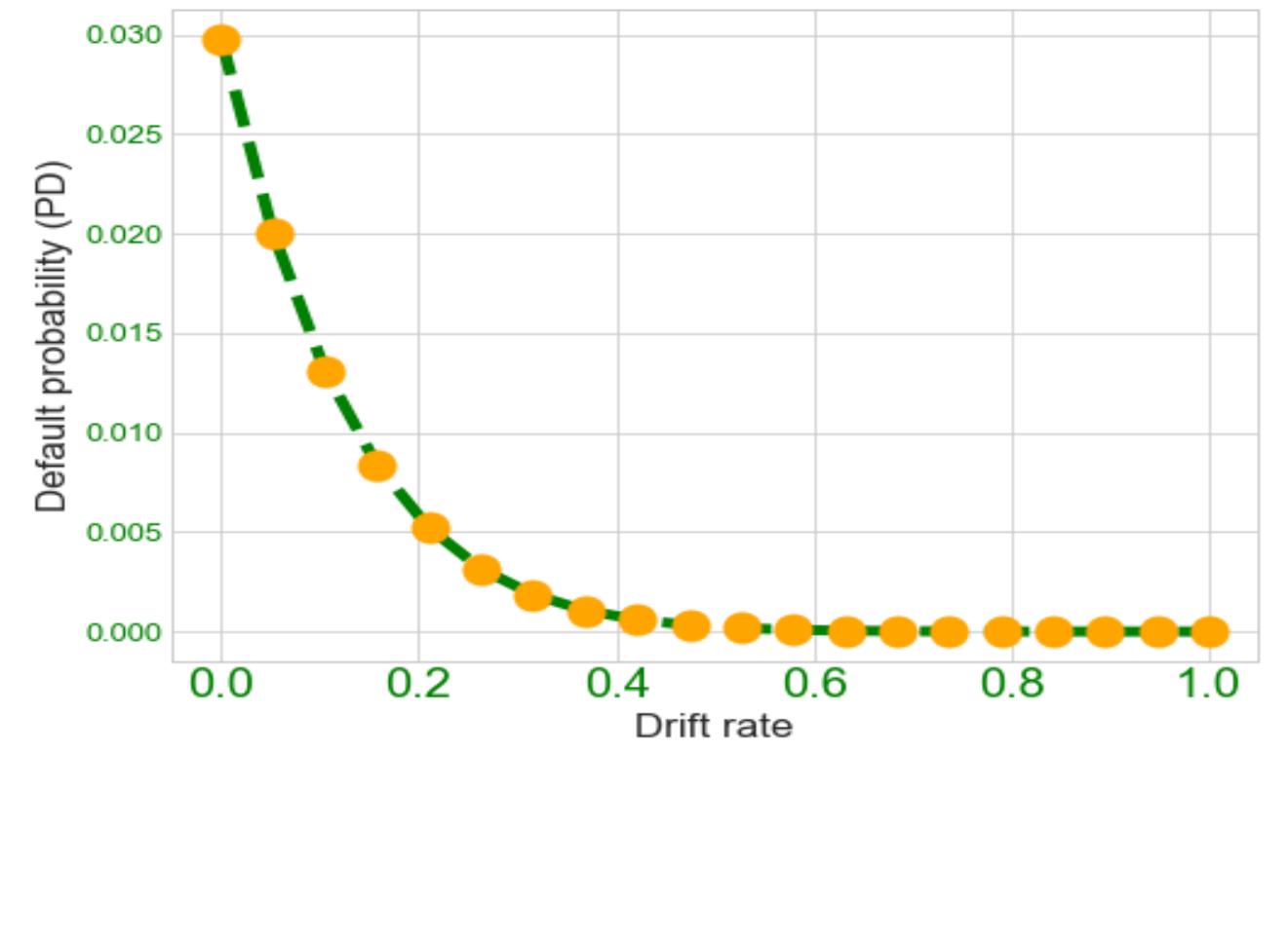
In our study we have come to know that if we plot the graph of default probability (PD) against an increasing drift rate while keeping all other parameters constant we will have the figure below.

Figure 4.3: Default Probability against Drift Rate

From Figure 4.3, we observed that a higher drift rate will produce a lower default probability. Coming back to Table 4.6, the risk-free rate of the asset iterate given as $R f=0.60 \%$ is comparatively lower than the drift rate $\mu=6.16 \%$ in Table 4.5. This explains why the actual default probability (APD) from Table 4.5 is quite low in value when compared to the risk-neutral default probability (RNPD) in Table 4.6. Thus, it makes sense to logically think that the RNPD is an upper bound for the APD since investors generally expect returns greater than the risk-free rate for holding a risky underlying asset. However, if the underlying asset drift at a risk-free rate then APD will be equal to RNPD hence the following inequality is true